Deep learning methods emerged in the 2010s and they showed impressive performance on image, text, and audio data. These methods are mostly based on artificial neural networks, which were first experimented with in the 50s. At the time, neural networks were mostly a research topic and not so much used for practical applications. Thanks to the speed of modern computers and to some algorithmic innovations, deep learning methods are now heavily used, in particular on perception and other unstructured data problems. Deep learning is an active field of research and one of the contenders to deliver human-like artificially intelligent systems.
This chapter will cover what deep learning is and detail its main flavors: fully connected networks, convolutional networks, recurrent networks, and transformer networks.
From Neurons to Networks
Deep learning means learning using an artificial neural network. Let’s look at the original formulation of neural networks to discover what they are.
Artificial Neuron
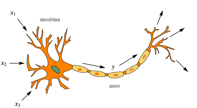
Artificial neural networks are inspired by what we know about the brain. In a nutshell, the brain is an information processing system that is composed of cells called neurons, which are connected together in a network. Neurons transmit electric signals to other neurons using these connections, and together, they are able to compute things that set our behavior. Humans have about one hundred billion neurons in their brains and about ten thousand times more connections. Here is a classic representation of what a biological neuron is:
On the left side we can see dendrites, which are branches from where the neuron receives its electric inputs (shown as x1, x2, and x3 here). The cell then “computes” an electric output (shown as y here), which travels along the axon and is sent to many other neurons (potentially thousands) through small junctions called synapses.
There is a large variety of biological neurons, and they perform different operations. They have in common that they “fire” sharp electric signals called spikes if some conditions in their inputs and internal states are met. Such analog computations are hard to simulate, and while there are many computation models of biological neurons, they are impractical for machine learning.
Artificial neural networks are not trying to mimic biological networks exactly. Instead, they use the same underlying principles while keeping things simple and practical (in the same way as planes are not mimicking birds). Artificial neural networks use artificial neurons, which are much simpler than their biological counterparts. Given numeric values x1, x2, and x3, the artificial neuron computes the following:
Here w1, w2, and w3 are learnable parameters called weights, which can be interpreted as connection “strengths” between neurons. This could correspond to the number of synapses between two biological neurons. b is another learnable parameter called a bias. In biological neurons, this value could be interpreted as a threshold above which the neuron fires. f is a nonlinear function called an activation function or transfer function. Biological neurons also use some kind of nonlinear activation function since they either fire or not. Here is an illustration of the computation made by this artificial neuron:
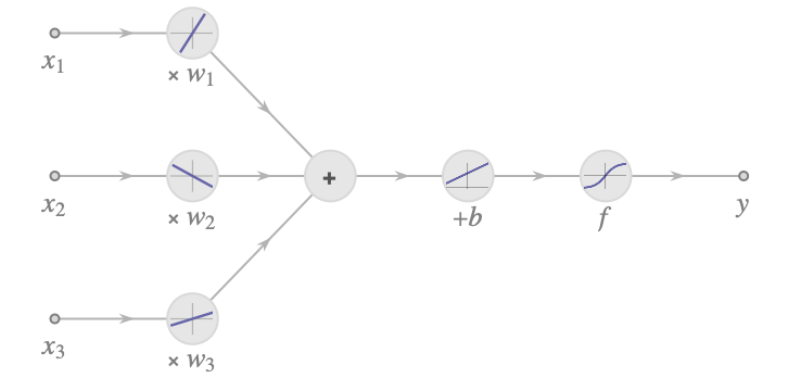
The first part is a linear combination of the features, and then a nonlinearity is applied. The presence of this nonlinearity is important. It allows neural networks to model nonlinear systems (because the composition of linear functions is still a linear function). Since biological neurons either fire or not, it is tempting to use some kind of step activation function. Historically, artificial neural networks used the logistic sigmoid function or the hyperbolic tangent function:
Note that with a logistic activation, this artificial neuron constitutes a binary-class logistic regression model. Modern neural networks have mostly moved away from such step functions. A classic modern activation function is the rectified linear unit, abbreviated ReLU:
While extremely simple, this activation function works pretty well in deep neural networks. Most modern nonlinearities are variations of the ReLU activation.
Modern deep learning models tend to depart from biological interpretations. However, they still, surprisingly, use the same principles described here: linear combinations of inputs followed by nonlinearities.
Classic Neural Networks
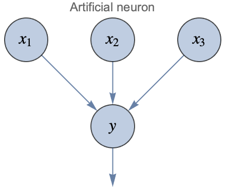
Now that we have an artificial neuron, we can use it to create networks by connecting many of them together. When part of a neural network, artificial neurons are often called units and are usually represented like this:
Circles represent numeric values called activations. It is implied that y is a linear combination of its inputs plus some bias term and that the result is passed through a nonlinearity. Following this convention, here is what an artificial neural network could look like with random connections between neurons:
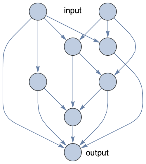
This network has two input values and one output value. Notice that the graph is directed and acyclic, so we can compute the output by simply following the edges.
This network is a parametric model. There is one weight parameter per edge and one bias parameter per neuron. We could train this network in the same way as any other parametric model: by minimizing a cost function computed on some training data (see Chapter 5, How It Works). Note that, contrary to what happens in biological neural networks, edges are not removed or added during the learning process; only the numeric parameters (weights and biases) are changed. It is possible to add/remove edges as well, but it is time consuming, so it is only done as a separate process to discover new kinds of neural networks (a process known as neural architecture search).
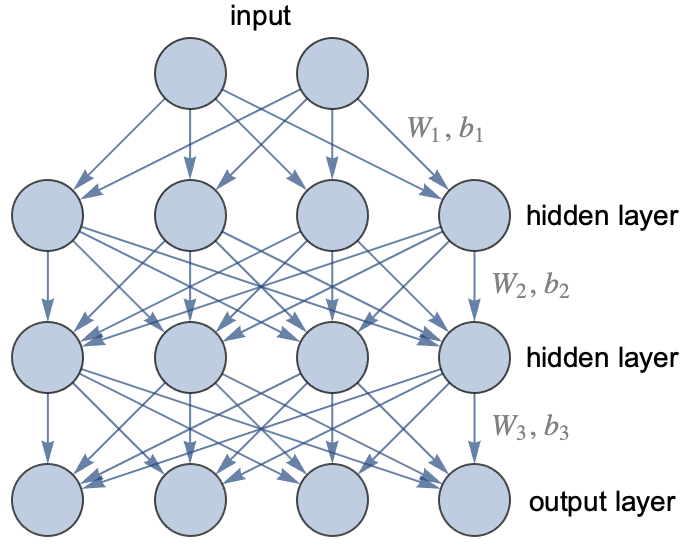
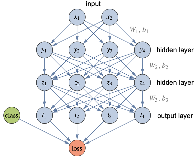
In practice, we do not use networks with random connections. Rather, we use a known architecture. A neural architecture is not an exact network but a class of neural networks sharing similar structures. The oldest and most classic architecture, invented in the 1960s, is called the multilayer perceptron or fully connected network, or sometimes feed-forward neural network. In this architecture, neurons are grouped by layers, and every neuron of a given layer sends its output to every neuron of the next layer (and only to them). These fully connected layers are also called linear layers or dense layers. Here is an example of such a network:
This network has three layers (the input is not really a layer): one output layer and two so-called hidden layers because they are only intermediate layers. This network takes two numeric values as input and returns four numeric values as output. It could be used to train a classifier that has four possible classes, and the output values would then be class probabilities. For a regression task, we would only have one output (the predicted value).
This layered architecture allows for the performance of several computation steps, like a classic program would, so it gives us the ability to do some reasoning. Most artificial neural networks have a layered architecture (and layers are also present in biological neural networks). In this illustration, two hidden layers were included, but there could be many more. A network with only one hidden layer or less is called a shallow network while a network with two or more hidden layers is called a deep network, hence the name of “deep learning.” This name highlights the importance of using models that can perform several computation steps.
In this graph, each arrow represents a weight. The first layer, therefore, contains 2×4=8 weights to compute the activation of the first hidden layer from the inputs. To these weights, we must add one bias parameter per output. These weights can be represented as a matrix. Let’s define and visualize random weights and biases for each layer:
We can compute the output of each layer using matrix multiplication. For a given input vector x and activation function f, the output of the layer i is as follows:
Let’s say that the activation functions are hyperbolic tangents for the hidden layers and that there is a softmax function at the end of the network, which is classic for a classifier (see the Logistic Regression section in Chapter 10):
The output of the network for the input x0={1.2,4.5} is thus given by:
This would correspond to class probabilities.
Note that most operations are matrix multiplications here. This is generally the case in neural networks. Modern computers are surprisingly good at multiplying matrices, and this operation can be parallelized to take advantage of multiple computing cores (such as the ones inside graphical processing units). The speed of matrix multiplication is one reason for the success of neural networks.
The multilayer perceptron is the original neural network architecture, but it never really managed to take over classic machine learning methods on structured data problems. In 2017 though, it had been shown that multilayer perceptrons can rival classic machine learning methods on structured datasets thanks to the self-normalizing architecture:
This network is a classic multilayer perceptron except that it uses dropout for regularization and, importantly, it uses a scaled exponential linear unit (SELU) activation function. This particular activation function happens to keep the activations in a given range, which allows the training of deep, fully connected networks.
The use of multilayer perceptrons is still marginal though. Neural networks are mostly used on unstructured data (image, text, sound, etc.) thanks to architectures such as convolutional neural networks, recurrent networks, or transformer networks. These architectures still use the concept of layers, but their connectivity is quite different from multilayer perceptrons.
Modern Neural Networks
Let’s now present a more modern view of what neural networks are. Nowadays, neural networks tend to be viewed more as graphical programs or even just as regular programs. Here is an implementation of the multilayer perceptron that we defined earlier (set up for a classification task):
We used ReLU activations here, and the last element is a softmax function to make sure that we output valid probabilities. The parameters are randomly initialized, so we can already use this network to obtain an output from an input:
Let’s look at the graph of the network in more detail:
This graph shows how the network performs its computation. As you can see, it is composed of several modules, such as ![]() , which are the layers of the network. Each layer performs a simple computation from its inputs and sends its output to other layers, as indicated by the edges of the graph. This is a graphical program, similar to a circuit.
, which are the layers of the network. Each layer performs a simple computation from its inputs and sends its output to other layers, as indicated by the edges of the graph. This is a graphical program, similar to a circuit.
In this case, the data flowing through this graph is numeric vectors (at first of length 2 and then of length 4 for the rest of the network). In the general case, neural networks can process matrices and even arrays of higher rank (the number of dimensions). These numeric arrays of arbitrary rank are often called tensors.
We can see two types of layers here. Some layers have circular borders, like ![]() , and this means that they perform a fixed operation. Other layers have square borders, like
, and this means that they perform a fixed operation. Other layers have square borders, like ![]() , and this means that they contain learnable parameters, which are often just called weights as a general term. A neural network is, therefore, a parametric model that processes numeric arrays in a circuit-like fashion.
, and this means that they contain learnable parameters, which are often just called weights as a general term. A neural network is, therefore, a parametric model that processes numeric arrays in a circuit-like fashion.
As with most other parametric models, training a neural network is done by minimizing a cost function. For classification, this cost would typically be the mean cross entropy (see Chapter 3, Classification). For regression, it would be the mean squared error (see Chapter 4, Regression). Let’s train a one-layer neural network on a simple regression task and visualize the learning curve:
This learning curve shows the value of the cost during the training phase. We can see that optimizing a neural network is an iterative process: the parameters of the network are modified step by step, in a way decreasing the cost. The parameters are actually modified together and in a continuous fashion, a bit like turning knobs in directions that reduce the cost (see the section How Neural Networks Learn in this chapter). One important aspect is that all layers are learned together, which allows for layers to collaborate in finding a good model. This also means that—if we have enough data—we don’t have to preprocess the data too much because the network can learn the entire model by itself. This is called end-to-end learning.
Neural networks are a flexible class of models. They can be defined to attempt to solve just about any kind of task (classifying things, generating text, generating images, etc.). There are several ways to define neural networks. The most classic way is to simply chain layers together, as we did before:
These chain networks are pretty common and easy to define. Sometimes a chain is not enough though, and we need to define more complex structures. This can be done by defining a set of layers and connecting them together in a graph:
This graphical network is also a valid neural network. While graphs are a nice way to visualize neural networks, programming with graphs can be cumbersome. An alternative approach is to use classic programs. Here is an example:
This program contains instructions and learnable parameters (defined by NetArray here), and it corresponds to the following graph:
This programmatic approach to define neural networks is often more convenient than defining layers and edges. Also, this approach allows for the inclusion of loops and conditional constructs, which are not common but can be useful nevertheless.
As for classic programs, there are high-level and low-level ways to define neural networks. When using low-level tools, we might need to construct most layers from scratch and specify their data type, their data dimensions, and how they are initialized. When using higher-level tools, we generally use built-in layers, and things like data type, array dimensions, or weight initializations are automatic. The networks defined here are using such high-level tools.
In practice, these networks can be pretty big and complex, so creating them from scratch is difficult even with high-level tools. The usual strategy is to take existing networks that have been created for similar tasks and to modify them. Such “surgical operations” can be done by directly modifying the source code or through specific tools. Let’s, for example, take the neural network of ImageIdentify from the Wolfram Neural Net Repository:
A classic operation is to change the number of classes returned and to replace the last layer because it does not have the correct dimensions anymore:
This process is typically done for a transfer learning procedure (see Chapter 2, Machine Learning Paradigms).
As we saw, the word “deep” in “deep learning” refers to the fact that we use deep neural networks, which means networks with many layers. Such deep networks perform several successive, simple computations, which allows for some sort of quick reasoning. This is in opposition to shallow machine learning methods, such as linear regression, which only perform one simple computation. This “computational depth” confers an advantage over shallow models for certain kinds of problems.
In a nutshell, deep learning methods work well for problems that involve a large number of variables (i.e. high-dimensional data) and, therefore, a large number of examples (unless transfer learning is used). More precisely, these methods are most useful when the meaning in the data emerges from complex interactions between variables. Let’s explain what this means using an image as an example:

By themselves, pixels have very little information about what is in this image. We could not identify this cat by having every pixel “voting” about what the object is, at least not without having them talking to other pixels. Rather, it is the interaction between many pixels—forming textures, shapes, etc.—that is informative. These patterns cannot be identified with a simple computation. Deep learning models can learn these patterns by making several simple computations. At first, they detect things such as lines by analyzing the pixels. Then, from these lines, they detect more complex shapes. Then, from these shapes, they detect object parts and so on until they can identify the main objects (see the section Convolutional Networks in this chapter for a visualization of this gradual understanding). This sort of staged detection process can work because the network is deep and also because images have a somewhat hierarchical or compositional nature. Images are not the only data type to be hierarchical/compositional. Audio, for example, is pretty similar. Text is as well: characters form words, which then form sentences, etc. The overall meaning emerges from complex interactions. Neural networks work pretty well for all these types of data.
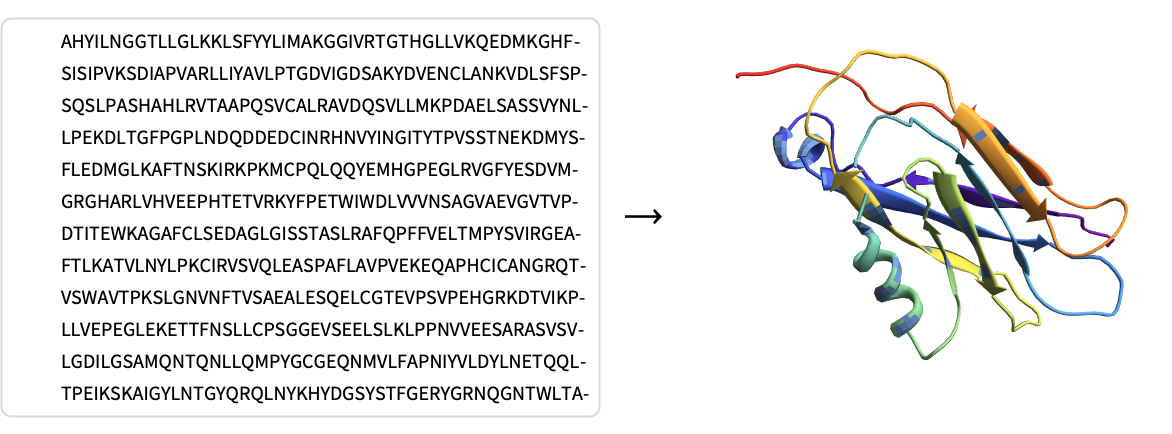
Neural networks are not limited to images, audio, and text though. They are, for example, used to play board games such as chess or Go by learning to predict if a game configuration is good or not. They are also used to speed up physics simulations, to predict if a molecule has a chance of being useful as a medicine, or to predict how a protein folds itself given its amino acid sequence:
While these tasks might appear different from perception tasks, they are also unstructured and have in common that the data is high dimensional and often displays some form of compositionality.
One thing to keep in mind is that current neural networks learn a particular kind of program. For example, these networks only process numeric arrays and cannot manipulate categorical objects, called symbols in this context. Also, they only learn a set of continuous parameters and do not learn usual programming constructs (loops, conditional statements, etc.). Such network programs can be very good at some tasks but not others. Overall, neural networks are pretty good at learning “intuitive” tasks. A rule of thumb is that if a human can perform a task in less than one second, it probably means that a network can do this task as well. If it takes longer than a second for a human to perform the task, it probably means that humans are using some kind of conscious reasoning, which deep neural networks are currently not very good at modeling.
While rather simple in nature, neural networks can get big in terms of the number of layers and parameters. Here is a visualization of every layer of the neural network of ImageIdentify:
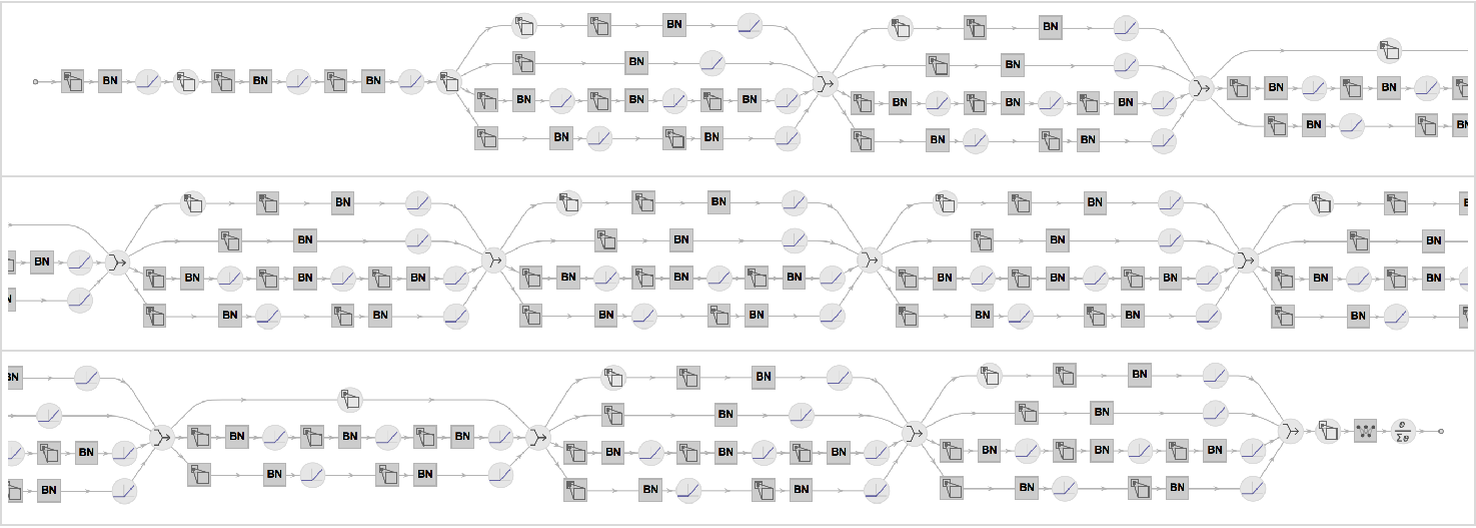
There are 232 layers of seven different types:
We can see some identical structures, which are referred to as blocks. Here is a visualization where “container layers” represent these blocks:
The hierarchy neuron layer block network is typical.
This network has about 15 million numeric learnable parameters, and this is not even a big network by modern standards. For example, GPT-3 is a language model trained in 2020 that has about 175 billion parameters. These sizes are inherent to the tasks they solve: recognizing images requires a lot of knowledge and so does generating text.
Since deep neural networks have many parameters, they require many training examples. Image identification networks are typically trained from tens of millions to hundreds of millions of images. The language model GPT-3 used a corpus of hundreds of billions of words. These datasets contain more data than any human has ever read, seen, or heard. One day we might discover networks with specific architectures that are more data efficient, but large datasets are currently essential to train deep neural networks unless we start with a pre-trained network, of course (see the Transfer Learning section in Chapter 2).
The drawback of networks being large and requiring a lot of training data is that the amount of computation needed to train them can be enormous. The solution is for networks to use simple and parallelizable operations. The bulk of neural networks computation is matrix multiplication. Computers and libraries are optimized to perform this operation quickly. For example, the following matrix multiplication requires about 1012 additions and multiplications but only takes 16 seconds on a standard laptop:
On this same laptop, evaluating the ImageIdentify neural network takes less than a 10 th of a second:
Part of this speed comes from parallelization. On CPUs (as used here), parallelization already helps, but we can obtain much better performance using chips like graphics cards (GPUs), which contain thousands of independent processing cores. Note that artificial neural networks, like their biological counterparts, are parallel computing systems at their core, so it makes sense that the best chips to train and use them are parallel computing chips. As of the early 2020s, GPUs are the most popular chips to train neural networks. We might expect specific hardware to take over and be even faster in the future. This high processing speed is central to deep learning and one of the reasons for its success.
Another reason for the success of deep learning is that we can modify the architecture of the network. For example, we can easily reduce the size of a network to trade accuracy for speed. More importantly, we can choose an architecture that is adapted to a given task, and this allows us to include knowledge that we have about this task. For example, convolutional neural networks are particularly well adapted for images and recurrent or transformer networks are pretty good at solving natural language processing tasks.
How Neural Networks Learn
Let’s now see how neural networks can learn. As with most other parametric models, learning is done by minimizing the cost function (see Chapter 5, How It Works), which is a sum over the losses of individual examples, plus some optional regularization terms. For a supervised learning problem, we can write this cost function as follows:
Here xi and yi are the input and output of example i, f is the network, and w are the parameters of the network. For regression problems, the loss would be the squared loss (see Chapter 5, How It Works), and for classification, it would typically be the cross-entropy loss:
Here Pw (yixi) is the probability that the network assigns to the correct class, so using this loss implies that the network will try to assign high probabilities to correct classes during its training. Let’s attach a loss function to the neural network classifier defined previously:

For this network, the probability Pw ( yixi) is the activation corresponding to class yi in the output layer.
During the training phase, neural networks average the loss of training examples and attempt to minimize the resulting cost function. Note that all the learning parameters of neural networks are continuous numeric values. It is a bit like having a set of knobs that we need to turn to obtain the lowest cost possible, and, hence, the best network. Many optimization procedures could, in principle, be used to do this. As it happens, the simple gradient descent method works best here thanks to the ability of neural networks to efficiently compute derivatives.
Gradient Descent
Gradient descent is a method to minimize functions that have continuous numeric inputs, like the cost functions of neural networks. The basic idea of the method is to start from an initial position and then keep following the steepest descent direction until we reach a minimum.
To explain this in more detail, let’s define a simple dummy function that we will try to minimize:
This function takes two values as input (which would correspond to the parameters of the network) and returns a number:
Here are visualizations of this function:
We can see high-valued regions in blue and low-valued regions in red, where the minimum must be.
How can we find where the minimum is? For some simple functions, it is possible to obtain an exact answer by doing a bit of math. For the cost function of neural networks, however, this is not the case, and we have to resort to approximation procedures. Gradient descent is one of these procedures.
To use the gradient descent method, we need to start from an initial position (that is, an initial set of parameters), say w1=1.5 and w2=2.3 in our case:
Then, we need to compute the derivative of the function with respect to the parameters at this initial position. This derivative is a vector called the gradient and is generally noted with the symbol ∇:
Let’s compute this gradient vector for any possible parameter:
At our initial position, the gradient is:
This vector tells us about the slope of the function cost in each direction. This means that near the position {w1,w2}={1.5,2.3}, increasing w1 by some amount increases the value of cost by 2.01 times this amount. Similarly, increasing w2 by some amount increases cost by 1.54 times this amount. Let’s display this gradient vector at the position for which it has been computed:
This vector indicates the steepest ascending direction, and we can see that it is perpendicular to the contour line, as it should be. Also, the magnitude of the vector indicates how steep the slope is.
Since we know the steepest ascending direction, we can go in the opposite direction in order to decrease the value of the function. But how far should we go? Indeed, this steepest descent direction is only valid at the position for which we computed the gradient, so if we move too far, we take the risk of increasing the value of the function. The classic strategy is to move proportionally to the gradient:
In this context, the step size α is called the learning rate because it controls how fast we attempt to learn. The learning rate α is a hyperparameter of the training procedure, and we can try several of them and pick the best one. Let’s use α=0.2, which means moving by 20% of the gradient magnitude:
Let’s compare the value of the function before and after the move:
The value is now lower. We made progress. Let’s display these two positions:
We can see that we got closer to the red regions. We could now compute a new gradient and perform another step. The gradient descent method simply repeats this process several times until the function value does not decrease much anymore.
Local and Global Minima
Let’s now perform 20 iterations of gradient descent starting from two different initial positions:
We used a learning rate of α=0.1 here. Let’s visualize the positions that we visited during the procedure:
As we can see, the trajectories follow the steepest slopes, like particles flowing downhill. After about 10 iterations, each trajectory reaches a stationary position, but we can see that these positions are different. Both of these stationary positions correspond to minima in the sense that everything around them is higher, but only one corresponds to the true minimum of the function. This true minimum is called the global minimum, and any other minimum is called a local minimum.
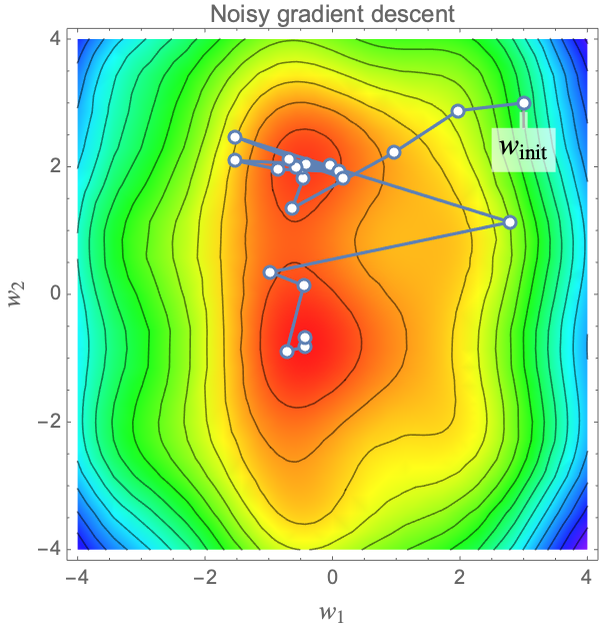
These local minima are one of the main issues of the gradient descent method for finding where the global minimum is. Indeed, because the gradient descent method only explores the function by doing small moves, it has a chance of getting stuck in a local minimum. This is why the gradient descent method is called a local optimization method. Global optimization methods, on the other hand, are supposed to find the global minimum, but they are generally slower than local methods. To augment the chances of finding the global minimum, we could, for example, start with many different initial positions or add some noise to the gradient to be able to escape local minima. Here is an example of such a noisy gradient descent, which is also similar to what happens when using stochastic gradient descent (see the section Stochastic Gradient Descent in this chapter):
For some simple parametric models such as linear or logistic regression, the cost function happens to be convex, which means that there is only one minimum. Such cost functions are easy to optimize using local optimization procedures like gradient descent. However, for deep neural networks, this is not the case; their cost functions have plenty of local minima, and finding their global minima is very difficult. Fortunately, this is not much of a problem. Before the deep learning “revolution” of the 2010s, neural networks were small and pretty hard to train, mostly because of this local minima problem (and of course, slow computers). These optimization difficulties were thought by many to be an insurmountable obstacle to scaling up neural networks in the future. As it happens, the opposite effect occurs: large neural networks have fewer local minima than we would think, and these local minima are not bad places to get stuck. They can even lead to better networks!
One intuitive explanation behind this is that large neural networks have many parameters, sometimes even much more than the total number of training examples (which is also the case for the brain). Because of this over-parametrization, there are many sets of parameters that give good networks for a given task, so it is easier to find one of them than it is to find a unique minimum. Also, the dimension of the cost-function space is so high that there is often a way out: even when the network seems to get stuck in a minima, one of the many directions might allow for escape. Finally, the gradient descent procedure is likely to end up in a local minima that has a large basin of attraction, and these kinds of minima are usually quite good (in a sense, gradient descent is adding an implicit regularization). Overall, if we initialize a neural network correctly (and we now have good methods for that), a simple gradient descent should be able to train it.
Learning Rate
We used a learning rate of α=0.1 before. Using a good learning rate is important. If the learning rate is too small, the convergence will be too slow, and if it is too large, the procedure might not even converge. Here are trajectories obtained with four different learning rates:

With a learning rate of α=0.5, the optimization converges but slowly. With α=0.2, the convergence is faster. With α=1, the optimization quickly finds the red regions but then does not converge. With α=1.5, things are even worse. The optimization diverges. This analysis is confirmed by looking at the cost values during the optimization:
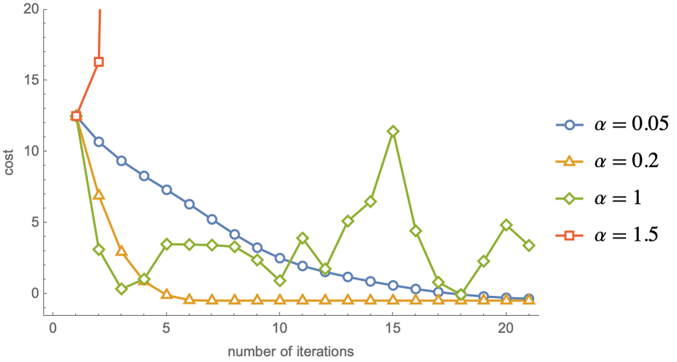
Clearly, α=0.2 is the best choice here. These curves are called learning curves (the same name as the curve showing the cost as function of the number of training examples).
For this specific problem, there is a transition from convergence to divergence for α=1, so we should pick a learning rate below this value. For other problems, such a transition might not be well defined; a learning rate might work well in some regions of the parameter space but might lead to divergence in other regions. To tackle this problem, it is possible to define a learning rate schedule; for example, we could start with a learning rate of α=0.01 and then switch to α=0.001 after some iterations.
A better solution yet is to automatically adapt the learning rate during the optimization. There are various methods to do this, such as adding a momentum to the optimization dynamic (the descent then behaves more like a ball rolling along the cost landscape). As of the early 2020s, the most popular method is called Adam. Most of these adaptive learning rate methods leverage the fact that when successive gradients are in the same direction, we should increase the learning rate, and when successive gradients are in opposite directions, we should decrease the learning rate. Another idea is to infer the local curvature using previous gradients and use it to make better step sizes.
Even with these adaptive methods, we still have to choose some kind of global learning rate (which is generally also called the learning rate). There are various empirical procedures to pick a good value for this hyperparameter, some of which involve continuously changing it during an optimization and checking how fast the cost is decreasing. This choice can also be automatized.
Stochastic Gradient Descent
There is one crucial difference between the vanilla gradient descent and the way modern neural networks are actually trained, and this concerns the way the gradient is computed.
Computing the cost function of a neural network is computationally intensive because we need to sum over all training examples:
The same problem occurs when computing the gradient:
If we have millions of examples, this is prohibitive. Fortunately, we do not need to compute an exact gradient to make progress. Indeed, since the cost function landscape is rather tortuous, the gradient does not indicate where the minimum is, so even a rough estimate of its value is useful, especially if we are far from a minimum.
One way to approximate the gradient is pretty straightforward: we use only a smaller set of training examples each time. For instance, we could randomly sample 100 training examples to compute the gradient at a given iteration, and for the next optimization iteration, we would sample another set of 100 examples. Each subset of training examples used is called a batch (or sometimes a mini-batch), and the overall method is called the stochastic gradient descent method (or mini-batch stochastic gradient descent method). Using stochastic gradient descent dramatically improves the optimization speed, which is why neural networks are always trained with this technique.
In practice, the random samples used are not independent from each other to avoid including the same examples in nearby batches. The usual way to implement stochastic gradient descent is to shuffle the data once and then to construct fixed batches of a given size:
Each batch is used to compute a gradient, and each gradient is used to perform one iteration of the optimization. The optimization cycles over these batches. Each time all batches have been visited, we say that the optimization performed a training round, or, more commonly, an epoch. Usually, several epochs are needed to train a neural network. Stochastic gradient descent is a form of online learning (see Chapter 2, Machine Learning Paradigms).
Let’s train a classic network on MNIST data (learning to recognize handwritten digits from 60000 images) for two epochs using a batch size of 128 and let’s visualize the learning curve:
We can see that the reported cost is noisy, which is normal because both the gradient and the cost are computed on single batches here. The average cost is overall decreasing.
One way to understand why stochastic gradient descent is faster than traditional gradient descent is to consider it from an information perspective; by learning in smaller batches, we make use of the information contained in these batches as soon as we process them. The closer we are to the minimum, the better the gradient is at indicating where the minimum is, so using the information contained in a given batch allows for better use of the information contained in the next batch.
Stochastic gradient descent introduces the batch size as a new hyperparameter. What value should we choose for it? This depends on the computer used. Let’s first assume that the throughput of a neural network (number of examples processed per second) does not depend of the batch size. Then, the optimal batch size is just 1. This might seem strange since using only one example per iteration leads to very noisy gradients, but we can compensate this by using a small learning rate. In the limit of small learning rates, reducing both the batch size and learning rate by the same factor should not change the optimization trajectory (if the examples are the same). Here is an illustration of this:
Also, using a single example per iteration allows us to make use of the information contained in this example immediately. This is why using a batch size of 1 is optimal, at least for such a computer.
In practice, however, the throughput of neural networks depends on the batch size. Here is the training throughput of the previous network as function of the batch size on a laptop:
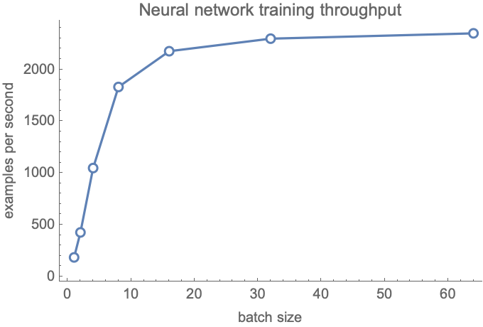
We can see a threshold around a batch size of 16 below which the throughput decreases. This is due to various latencies and less effective parallelization when a small number of examples are processed together. Such behavior is why batch sizes such as 32, 64, or 128 examples are frequently used. Another reason why we might want to increase the batch size is when some operations are explicitly performed on a batch as opposed to single examples. A classic example of this is the batch normalization operation (see the section Convolutional Networks in this chapter).
Besides being much faster than regular gradient descent, stochastic gradient descent offers a few extra advantages. One of them is that it is easy to work with datasets too large to fit in the memory since we only have to load one batch per iteration. Another advantage is that stochastic gradient descent sometimes allows for the escape of local minima thanks to its noisy nature. Finally, stochastic gradient descent adds an implicit regularization, which can allow for better generalization.
As of the early 2020s, just about all neural networks are trained with the stochastic gradient descent method.
Symbolic and Numeric Differentiation
Neural networks are trained using (stochastic) gradient descent. This means that, at each iteration of the optimization, we need to compute the derivatives of the cost (a.k.a. the gradient) with respect to each parameter for the current set of parameters:
There is an efficient method to compute these derivatives that is called backpropagation that will be presented in the next few sections, but to understand what backpropagation is, let’s first take a step back and see what derivatives are and what the classic methods to compute them are.
Let’s first define a simple sine function:
The derivative of this function at a given point is its current rate of increase (or slope). Let’s compute a numeric approximation of this slope at the position x0=1.2:
Let’s visualize the function and a line passing by (x0,f(x0)), whose slope is the derivative we just computed:
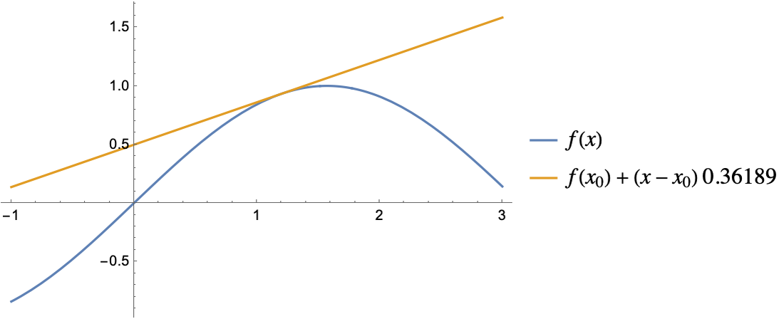
The line is tangent to the function, which means that our derivative is approximately correct. The method we used to compute this derivative is called numerical differentiation, also known as the method of finite difference. More formally, this method computes the derivative as
where ϵ is a small number.
If the function f has many inputs, we need to compute this difference independently for each input. For the first input, we would need to compute
For the second input, we would need to compute
And so on. Overall, the function f has to be evaluated as many times as the number of inputs, which is the number of parameters for us, so for a neural network of 15 million parameters, computing the derivative in such a way is about 15 million times more costly than evaluating the network once. Needless to say, this method cannot be used to train neural networks (at least in this naive form).
Another classic method to compute derivatives is called symbolic differentiation. The idea is that if a function can be written as a symbolic expression (a mathematical formula), we can differentiate this formula by applying some rules. For example, the symbolic function Sin would be transformed into the symbolic function Cos:
Neural networks are a composition of many functions. Let’s create a composition of 10 simple functions:
Let’s now see what symbolic differentiation returns for this function:
The result is a big formula that has 74 terms and is, therefore, quite a bit slower to evaluate than the original formula. This phenomenon gets worse with the size of the composition: for 100 composed simple functions, the symbolic derivative has about 5000 symbols:
In this case, the size of the symbolic derivative seems to scale like the square of the size of the original expression. This size is mostly due to repetitions of the same subexpressions over and over again because symbolic expressions are not like regular programs; they cannot store things in variables. Another issue with this approach is that it only works for symbolic expressions and not for arbitrary programs. As for numeric differentiation, this approach is not practical for computing the derivative of the cost function of a neural network.
Chain Rule
Let’s now look at the chain rule, which is a formula to efficiently compute the derivative of composite functions. The chain rule is a key element to differentiating neural networks.
If f and g are two functions of a unique variable, then the derivative of the composite function f(g(x)) is the product of f and g
This formula is easier to understand using Leibniz’s notation (here f and g represent the output values of the functions f(g(x)) and g(x)):
We can use this formula for arbitrary long compositions. Let’s apply it to the composition of these 10 simple functions:
The composite function corresponds to the following pipeline:
To apply the chain rule, we first need to symbolically differentiate each of these functions separately, which is fast because they are simple. Here are their corresponding derivatives:
Now let’s say that we want to know the derivative for the input x0=1.2. First, we need to compute all the intermediary values in the pipeline:
We can then compute the derivative of each intermediary function at their corresponding input:
Finally, we need to multiply these intermediary derivatives to obtain the overall derivative:
And that’s it. Let’s compare this value with the one obtained through symbolic differentiation:
The results are identical. The advantage of computing the derivative in this fashion is that we only performed about 20 operations (plus a sum), as opposed to more than 70 operations needed with the symbolic derivative. This ratio gets even larger for longer chains of functions. With this method, the number of operations needed scales linearly with the number of intermediary functions (as opposed to quadratically with symbolic differentiation), so computing the derivative of a composite function is only a few times slower than computing the function itself.
Chain Rule for Vector-Valued Functions
We have applied to chain rule for a composition of functions that have only one input and one output each. Let’s now see how we can apply it to functions that can have many inputs and many outputs and for which the last output is a unique number. This is similar to the layers of a neural network with a loss function attached at the end. Let’s use the following chain of functions f(g(h(x1,x2,x3))):
The function h transforms the vector {x1,x2,x3} into the vector { y1,y2,y3}, which is then transformed into the vector {z1,z2,z3} by the function g and, in turn, transformed into the scalar (i.e. single) value t by the function f. This could correspond to the following neural network:
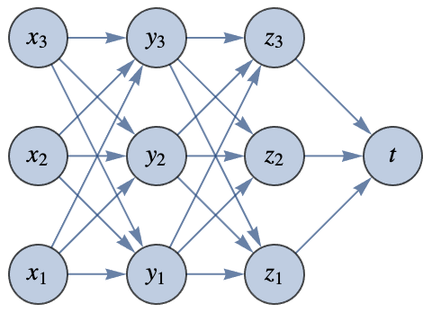
So we want to compute the derivative of this composite function, which is the gradient vector:
Let’s write this gradient in a way that will make the chain rule clearer:
The function f has multiple inputs and only one output, so its derivative is a gradient vector:
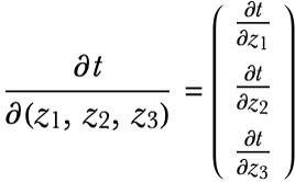
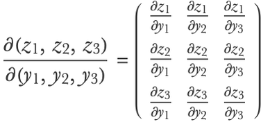
The functions g and h, however, have multiple inputs and outputs. Their “derivatives” are, therefore, matrices called Jacobian matrices. Here is the Jacobian matrix for the function g:
Compositions of such functions also have their chain rule. We can obtain the composite derivative by combining the gradients/Jacobian matrices of intermediate functions using matrix multiplication:
To apply this formula, we would first compute the values xi, yi, etc., then compute the gradients/Jacobian matrices of each function for these specific values and then combine these derivatives. Let’s generate synthetic values for these gradients and Jacobian matrices:

Now here is the important part: in order to compute the result efficiently, we should first multiply the vector with its corresponding matrix instead of multiplying the two matrices first. Here would be the full step-by-step computation:
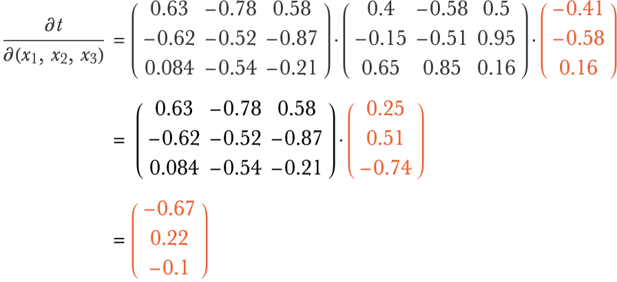
If we had a longer chain of nested functions, we would continue multiplying the vector with its nearby matrix.
Always multiplying the vector first allows for the avoidance of multiplying two matrices at any point, which would be slower. The effect is more important if the matrices are large. Let’s say that we have matrices of size nn and a vector of size n. The number of computations needed to multiply two matrices of this size is around n3, while it is only around n2 when multiplying a vector with a matrix. By using this computation order, we are effectively propagating the gradient from the end of the computation chain to the beginning of the chain, which is why it is called the backpropagation method.
Backpropagation in Neural Networks
We have seen how to efficiently combine the intermediate derivatives of composite functions with the backpropagation method. Let’s now see how we can apply backpropagation to neural networks.
Here is the multilayer perceptron that we defined before with its loss attached:
We are interested in computing the gradient of the loss with respect to the parameters (bi and Wi). Here is the computational graph of this network:

The parameters have square borders and the operations are circles. Each edge represents an array of numbers flowing through the graph. As we can see, the computation is not a simple chain: there are several “sources” (the input, the class, and the parameters), and there can be more that one input or output per node. This is a directed acyclic graph.
We can still apply the backpropagation algorithm in such a graph. As before, we would first evaluate the neural network and store all the activations obtained (one array per edge). This is called the forward pass. We would then start by computing the gradient of the loss with respect to the previous activation and backpropagate this gradient through the entire reversed graph (each edge is reversed). This is called the backward pass. The only condition for this backward pass to be possible is that each operation should be able to provide gradients with respect to its inputs when given gradients with respect to its outputs. Also, when two edges are merged (in the reversed graph), we simply add their gradients.
At the end of this backpropagation procedure, we would obtain the derivative of the loss with respect to every edge of the graph, including the parameters. Here are the loss gradients obtained for the input x0=(1.2,4.5), the class 3, and the parameters as defined earlier:
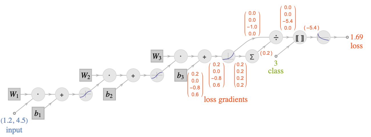
The gradient for the parameter vector b1 would be the vector (0.2,0.0,-0.8,0.6) (values are rounded), and we could use this to update the value of this parameter vector (along with other parameters) through a gradient descent procedure.
One important property of this algorithm is that for neural networks, the backward pass is at most a few times slower than the forward pass. This means that computing the gradient of the loss with respect to the parameters is about as fast as evaluating the network itself! This is quite impressive when considering how slow it would be to compute an approximate gradient using a method such as finite differences or symbolic differentiation. This ability to obtain a gradients cheaply justifies the use of the gradient descent method, and it is a key for the success of neural networks.
Backpropagation is a special case of the automatic differentiation method, which deals with computing derivatives of arbitrary programs. In our case, backpropagating the gradient is the optimal strategy because the output of the function is a scalar (the loss value). To compute the derivative of a function that has many outputs, we might have to propagate derivatives in another way (a mix of forward and backward propagation).
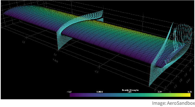
Another interesting aspect of backpropagation (and automatic differentiation in general) is that it can be used on programs that contain loops, conditional statements, and so on. To do so, we would first execute the program and store its trace (i.e. its computational graph for this specific execution) and then apply automatic differentiation to this graph. Such ability allows us to obtain derivatives of arbitrarily complex programs and opens up applications beyond neural networks. For example, we could optimize the shape of a wing by running a fluid simulation and computing the gradients of the drag and lift with respect to some parameters of the wing through the entire simulation:
In the early days of deep learning, practitioners had to implement their own backpropagation algorithm and define the derivatives of every operation they used in their network. Fortunately, this time is over. Nowadays, there are various neural network frameworks that can automatically differentiate any network or program that we implement and run on fast specialized hardware, such as GPUs.
Convolutional Networks
Let’s now introduce convolutional neural networks (also known as CNN or ConvNet), which is one of the most classic and fundamental neural architectures.
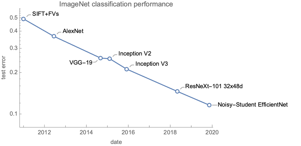
Convolutional neural networks are originally inspired by the visual cortex of animals and are particularly good for computer vision tasks. A classic task on which they excel is image classification. Before the 2010s, image classification was tackled using hand-engineered features and classic machine learning methods. This strategy only resulted in marginal improvements over the years. Since the 2010s, convolutional neural networks have changed this paradigm and led to important progress. Here is the state-of-the-art performance of models (at the time of their release) on the classic ImageNet classification task:
Every model here but the first one is a convolutional neural network. Even though these networks are convolutional, we can see that they don’t have the same performance. Most of these gains come from using better networks (and a part comes from using additional data and better training techniques). As of 2020, there are still improvements being made to the convolutional architecture.
Convolutional neural networks are not exclusively used on images. For example, they are used to process sequential data such as text, audio, and time series. Another domain of application concerns graphs, especially processing molecules. Finally, convolutional neural networks are sometimes used to tackle exotic tasks, such as playing board games.
Simple Convolutional Network
The main component of convolutional neural networks are convolutions. In the context of neural networks, a convolution is a linear operation making use of a moving window. The simplest example of such a convolution is a moving average over a list of values. Let’s compute the moving average with a window of length 3 for a sequence of five values:
Now, let’s compute a weighted average, using a weight of w1=1 for the first value of the window, w2=2 for the second one, and w3=3 for the third:
This is basically what convolutions are in neural networks: weighted moving averages. One difference is that, by convention, a weighted sum is used instead of an average:
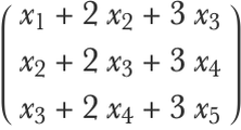
Another slight difference is that a bias term is added, such as:
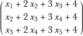
This convolution operation is equivalent to multiplying the input by a band matrix and adding a bias:

The moving window and its parameters {w1,w2,w3,b} are called a convolution kernel or convolution filter. Here is an illustration of the convolution procedure for an input of 10 numeric values (without bias here):

The symbol “⋆” represents the convolution operator. The kernel size is 3 here. Note that the output is smaller than the input. We can obtain an output of the same size by padding the input with zeros:

Such zero-padding is commonly used. Another variant is to move the window by steps larger than 1. Here is what we would obtain with steps of length 2:

This step size is called the stride of the convolution and, like zero-padding, is used to control the output size.
Okay, so let’s see how we can construct a network out of this operation. The simplest thing we can do is to stack convolutions and alternate them with nonlinearities. The learnable parameters would be the kernel weights and biases. Since the convolution operation is linear, we can represent the network in the same way as we did for multilayer perceptrons. Let’s show a convolutional network (with a kernel of size 3 and some zero-padding) and a fully connected network side by side:
We can see that convolution layers are quite different from fully connected layers. In a fully connected layer, every input is connected to every output. In a convolution layer, however, only “nearby neurons” are connected. The connections are thus sparse and local. The other important difference is that many connections use the same weights (each color represents one weight here). We say that weights are shared. As a consequence, convolutional networks have far fewer parameters per layer than fully connected networks for a given number of neurons. In this illustration, the fully connected network has 5×5=25 weights and five biases per layer while there are only three weights and one bias per layer for the convolutional network. This ratio can get much bigger when there are more neurons per layer. Note that since the kernel of convolution layers has a finite size, these layers cannot extract information resulting from the interaction of elements far apart. Stacking several layers solves this problem. Deep kernels can indirectly see the complete input; their effective receptive field is large.
This specific connectivity of convolutional networks is the reason for their success. Let’s try to understand why. The idea is that the connectivity of convolutional networks carries implicit assumptions about the data, which happen to be quite valid for data such as images, text, and audio. Because these assumptions are valid, we don’t start from scratch, and we can learn using less data. These implicit assumptions are known as the inductive bias of the model (see Chapter 5, How It Works) or, in a Bayesian context, as the prior belief/knowledge that we have (see Chapter 12, Bayesian Inference).
For convolutional networks, the first implicit assumption is related to the local connectivity of the neurons. By only connecting nearby neurons, we assume that the input values are not in a random order and that there exists local patterns that are useful for understanding the data. This is true for images: objects are localized in a region of an image and do not involve every pixel. This is also true for text: nearby characters form words. This assumption is know as a spatial locality assumption.
The second implicit assumption is related to weight sharing. By using the same weights everywhere, we assume that the meaning of patterns does not depend on their position. Again this is true for images: a bird is still a bird whether it is displayed on the left or on the right of an image. Similarly for text, the meanings of most words do not depend so much on their position in a sentence (not perfectly true though). This assumption is know as a translation invariance assumption (or shift/space invariance).
Because of these assumptions, convolutional neural networks obtain much better performance than multilayer perceptrons on images, text, audio, and all kinds of other data types. For classic structured data, however, this architecture does not provide benefits because these assumptions would generally be wrong. Another interesting aspect of this architecture is that it can process examples that have varying lengths (the output of each layer would also be of varying length), which is useful for working on text and audio.
2D Convolutional Networks
In the previous section, we introduced a convolutional network that takes a vector as input. Such a 1D convolutional network could be suitable to process audio or text but not images since images have two spatial dimensions. Let’s see how we can adapt our previous network to work on images.
Let’s start with grayscale images. As we saw before, images can be seen as an array of pixel values. In the case of a grayscale image, this array is just a matrix. Here are the pixel values for a 2828 image:
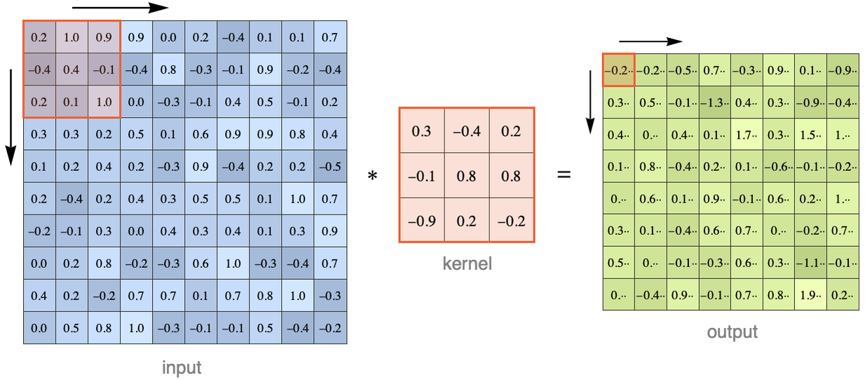
In principle, we could apply a 1D convolution to this matrix by “flattening” its values into a vector. The problem is that we would lose some spatial information. A better way is to use a 2D convolution. This can be done exactly like before except that the kernel is now a rectangle and that it scans the image in both directions. Here is an illustration for a kernel of size 33 applied to a 1010 matrix:
Here we can imagine the kernel window going from left to right, one pixel at a time, then going to the next line when the right border is reached, and so on (these operations can be done in parallel though). At each step, the corresponding input values are multiplied elementwise with the kernel values and then summed to obtain the result. A bias might also be added. Here is the computation made to obtain the value highlighted in red:

Note that the output of this convolution is a matrix and not a vector like before. In our case, the output is a bit smaller than the input. Again, we can add zero-padding to the input if we want to or use a different stride.
Now let’s see how we could define a convolution that can process a colored image. Colors are usually encoded as a vector of values. The most common encoding is the RGB encoding in which colors are a mixture of red, green, and blue:
Here are the dimensions for the pixel values of an RGB-encoded image:
As you can see, the pixels are not organized in a matrix of values but in a matrix of vectors, which means an array of rank 3. This new non-spatial dimension is referred to as the channels of the image. In this case, there are three channels.
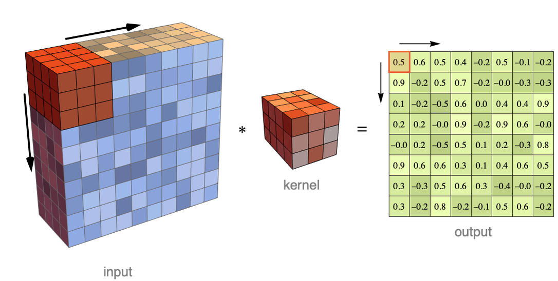
Okay, so we can adapt the previous convolution to work on this data as well by using a three-dimensional kernel that reads all the channels at once. Here is an illustration for an image that has four channels:
As before, the corresponding input values are multiplied elementwise with the kernel and then summed (and a bias might be added as well). In this illustration, this would mean that each output value is computed from 3×3×4=36 input values. This is still a 2D convolution because the kernel window is only displaced over the two spatial dimensions. As before, the result is a matrix (and again we can use padding or a larger stride).
We could create a network out of this operation by stacking convolutions and alternating them with nonlinearities. The learnable parameters of this network would be the weights and biases of each kernel. However, this network would be rather limited because it only uses one kernel per layer, which means very few parameters. In order to increase the number of parameters, the usual procedure is to use many kernels for each layer. Each kernel produces a matrix as a result, and the matrices are joined to form an array that has both spatial and channel dimensions. Here is an illustration of this operation:
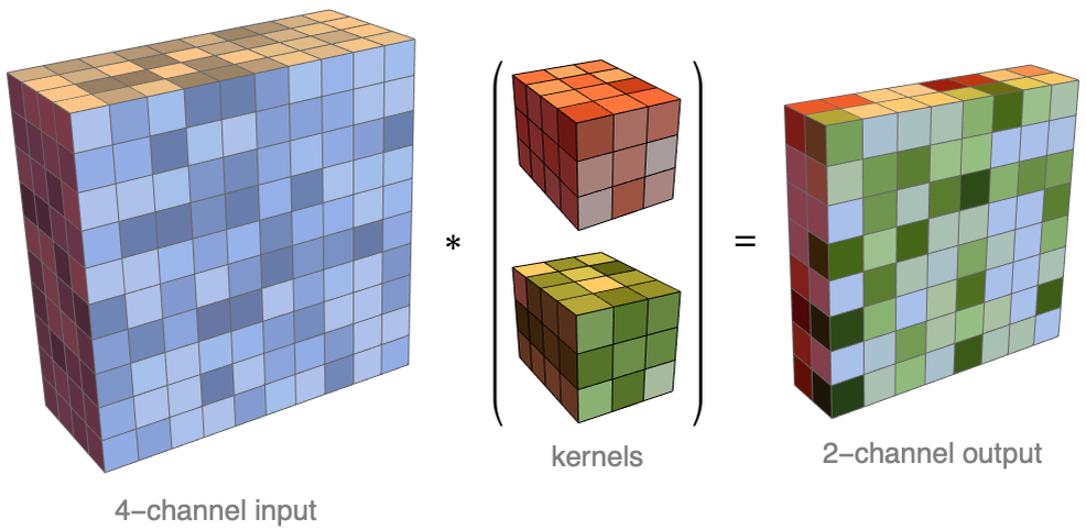
Each kernel produces a channel of the output array. Such a channel is also called a feature map because it represents the same feature computed at different locations of the input. In this case, the input has four channels and the output has two channels. Here is how we could define this convolution as a neural network layer:
We specified the number of output channels (2), the dimensions of the kernel (33), and the dimensions of the input (4410).
In practice, convolution layers have more output channels. Here is the first convolution layer of an image classification network called ResNet (residual neural network architecture):
This layer has 64 output channels and uses 77 kernels. Here are the weights of the kernels:
Since each kernel has three channels, we can visualize them as colored images:
We can recognize simple shapes such as lines in various directions and dots. These shapes are the first things identified by the network, and they form the features that are given to the next layer of the network. We can interpret each of these kernels as a detector that focuses on one kind of feature (hence the name of feature maps for their output).
Such a convolution layer is at the core of every convolutional neural network processing images.
LeNet
Okay, so now that we have defined 2D convolution layers, let’s see how they can fit into a network that processes images. We will start with the seminal LeNet neural network developed in 1989. This simple network was designed to classify handwritten digits. We can define this network by chaining several layers together:
Besides layers, you can see that this network also has a preprocessor to convert the input image into an array of values and a post-processor to convert the output probabilities into a class. Let’s apply this randomly initialized network to an image:
As expected, the result is wrong since this network has not been trained.
Before training the network, let’s analyze how it is constructed. This network has three learnable layers (and eight other layers, including the nonlinearities), with a total of about 400000 numeric parameters:
This is quite small by modern standards (this network only requires 1.7 MB of memory).
The first layer is a convolution layer with a kernel of size 55, and then there is the Ramp function, which is a rectifier nonlinearity (we replaced the original nonlinearities with something more modern). So far, nothing surprising. The next layer is new to us. It is a pooling layer or, in this case, a max-pooling layer:
This layer is a sort of “moving maximum” function: it uses a moving window like a convolution, but instead of performing a linear operation, it takes the maximum of all the values it reads. Pooling layers have no parameters and are typically used to reduce the resolution of the data by using a stride larger than 1. The next layers are again a convolution, a nonlinearity, and a pooling layer. Then, the data is flattened into a vector (FlattenLayer), processed by fully connected layers, and passed through a softmax function at the end. To summarize, this network starts with convolutions (plus max-pooling) and then switches to process vectors like a classic multilayer perceptron would. Let’s now look at the dimensions of the data inside the network:
We can see that the spatial dimensions (the last two numbers) are progressively reduced from 2828 at first, to 1212, 88, 44, and then 11 in the end. The number of channels (that is, the number of feature maps) increases from 1 to 800 and then decreases down to 10 because it is the number of classes. To better visualize these dimensions, here are the arrays that the network computes during its evaluation (with removed arrays having the same dimensions):
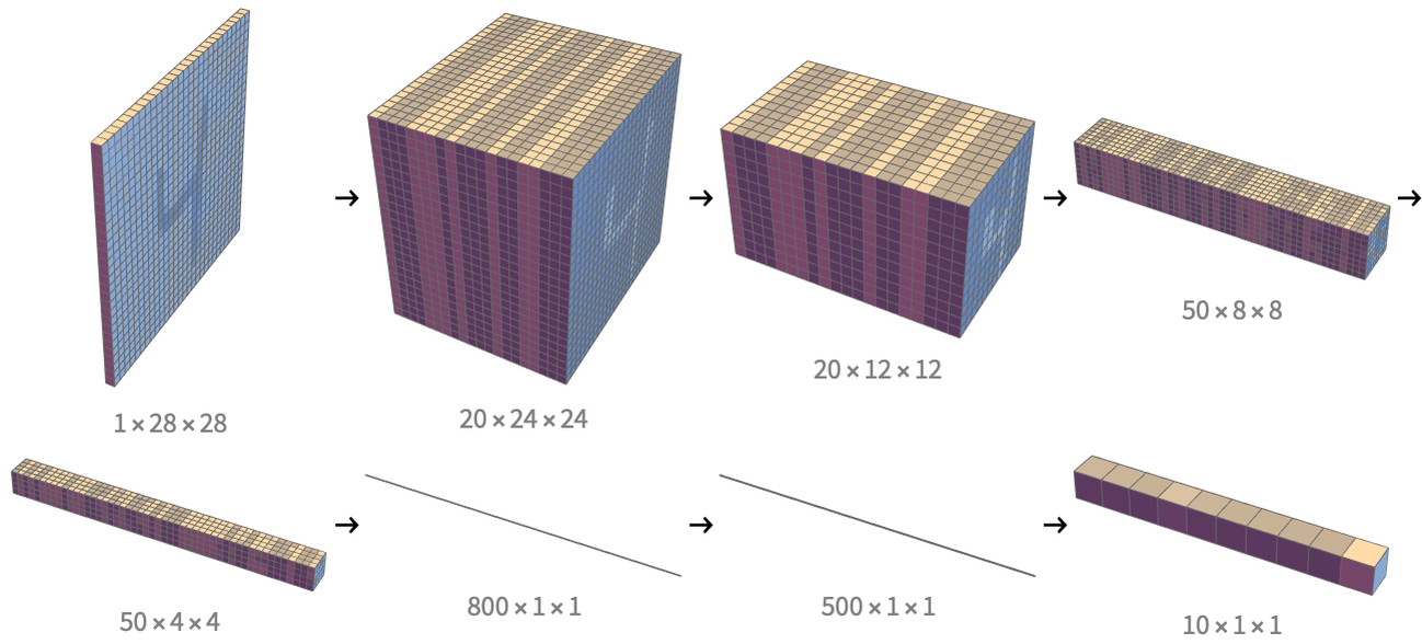
We can see how the spatial dimensions are gradually reduced and how the number of feature maps increases and then decreases. One interpretation is that the spatial information is gradually replaced by semantic information. Note that in the last array, only the last value is active, which means that the network believes the input is a 9.
Okay, so let’s now train this network. We use the handwritten digits of the MNIST dataset:
Here are 10 examples from this dataset:
First, let’s separate these 60000 examples into a training set and a validation set:
We can now train the network on the training set and use the validation set to monitor the progress. For this training, let’s also specify a loss function (the cross-entropy here), a number of epochs, and a batch size:
The network has been trained for 10 epochs. We can see that the training cost is decreasing, which is a good start. The validation cost is also decreasing at first, so the network learns something. Then, the validation cost seems to plateau and even increases sometimes, so we would probably not gain anything by training further. Adding regularization might help here (see Chapter 5, How It Works). We can also see that the Adam optimization method is used (the initial learning rate has been determined automatically).
Let's now extract the trained network and try it on validation examples:
This time, every example is correctly classified. We can also obtain class probabilities:
The network is very confident that it is a 6. Let’s now measure the performance of this network on the validation set:
We can see that this network performs pretty well: 99.6% of examples are correctly classified. The most common confusion seems to be some 7s being misclassified as 1s.
Modern Image Classifier
Let’s now analyze a more modern network such as EfficientNet, which, in 2020, obtained the best performance on the ImageNet classification task. Training this network on the ImageNet dataset would be quite slow and require special hardware (such as GPUs), so we will only analyze the following trained network:
This network is the smallest version of the EfficientNet family of eight networks. The largest contains 70 million parameters, needing about 280 MB of memory, while this one only contains about 5 million parameters, which fits into 21 MB of memory:
Let’s look at the types of layers present in this network:
As expected, there are convolution layers, elementwise layers (the nonlinearities), linear layers (the fully connected ones), and layers to perform simple mathematical operations. There are also two new important kinds of layers here: dropout layers and batch normalization layers.
Dropout layers are there for regularization purposes. The idea of dropout is to randomly “drop” activations during the training phase, which means that some activations are randomly set to zero and the others are multiplied by a constant factor to compensate. Here is the behavior of a dropout layer during the training phase:
In this case, each activation had a 50% chance of being dropped and a 50% chance of being doubled. During the inference phase, nothing happens:
Dropout pushes neurons to learn by themselves, as opposed to collaborating with other neurons. In a sense, it pushes the network to find simpler solutions. This method regularizes networks quite well, and it has been suggested that the brain is using some kind of dropout for regularization purposes.
Batch normalization layers are there to help train the network by making sure that activations are normalized (zero mean and zero variance) across the examples of a batch. This is a bit of a strange layer because during training, it acts on a batch, which means that examples are not processed independently (this behavior is quite unique). During the inference phase, however, it acts like a regular layer: the output of each example only depends on the input example. Batch normalization is very effective at stabilizing the training of a neural network, but there are controversies as to why this is the case. Also, it has some undesirable properties, such as being slow to compute and causing the batch size to influence the result. As of 2020, batch normalization is still present in most image classification models.
Let’s now look at the architecture of the network:
As we can see, this network is a chain containing several blocks. If we look at the activation dimensions (on the right side of the summary), we can see a similar pattern to LeNet: the spatial dimensions are progressively reduced from 224224 to 11 and the number of channel/feature maps is increased from 3 to 1280 and then reduced to 1000, the number of classes. Again, this makes sense since the network needs to convert spatial information into semantic information.
Let’s analyze one of the blocks of this network:
We can see that this block is composed of convolution layers, batch normalization layers, and nonlinearities. The important thing to notice about this block is that there is a sort of shortcut called a skip connection: the input is added back at the end of the block. This is called a residual block and was introduced as part of the residual neural network architecture (a.k.a. ResNet) in 2015. This fundamental innovation allowed for much deeper training of networks than before and improved the overall quality of networks. The idea behind this skip connection is that it makes it easy for the block to learn the identity function by just setting the weights to zero, which is necessary if the network is too deep. In a sense, the identity is the “default” behavior, and this is a good inductive bias. We can interpret such a residual network as iteratively modifying the input, almost like in a continuous transformation. Residual blocks are present in most modern neural networks, not just convolutional ones.
Inside this residual block, we can see a sub-block (![]() ) that is not convolutional. Let’s visualize it in greater detail:
) that is not convolutional. Let’s visualize it in greater detail:
This is called a squeeze-and-excitation block and was invented in 2017. This block looks like a residual block because there is a skip connection, but it is actually quite different because the input is multiplied back instead of being added back. The first layer (![]() ) is removing the spatial dimensions by computing the mean of every channel (480 channels here). This is called the squeeze operation. Then there is a multilayer perceptron (with a bottleneck like an autoencoder) that computes for each channel a “score” between 0 and 1 (note the last nonlinearity is a logistic sigmoid). This is known as the excitation operation. Each of these scores is then multiplied back with the corresponding input channel. This is an example of a gating mechanism, as in the LSTM architecture (see the Recurrent Networks section in this chapter), or, more precisely, a self-gating mechanism because the input is also used to compute the scores. Here, the squeeze-and-excitation block is choosing which channel should be set to zero and which one should be let through depending on the mean activation of every channel. This allows for directly modeling correlations between channels, which means correlations between shapes, objects, etc. (e.g. if a street is detected, a motorbike is more likely to be present than a dolphin). Squeeze-and-excitation blocks are very common in modern convolutional networks.
) is removing the spatial dimensions by computing the mean of every channel (480 channels here). This is called the squeeze operation. Then there is a multilayer perceptron (with a bottleneck like an autoencoder) that computes for each channel a “score” between 0 and 1 (note the last nonlinearity is a logistic sigmoid). This is known as the excitation operation. Each of these scores is then multiplied back with the corresponding input channel. This is an example of a gating mechanism, as in the LSTM architecture (see the Recurrent Networks section in this chapter), or, more precisely, a self-gating mechanism because the input is also used to compute the scores. Here, the squeeze-and-excitation block is choosing which channel should be set to zero and which one should be let through depending on the mean activation of every channel. This allows for directly modeling correlations between channels, which means correlations between shapes, objects, etc. (e.g. if a street is detected, a motorbike is more likely to be present than a dolphin). Squeeze-and-excitation blocks are very common in modern convolutional networks.
Overall, the architecture of EfficientNet is a bit more complicated that the one seen in LeNet. This is not surprising since the network is more recent. The precise architecture of this network (number of layers, type of nonlinearities, position of some blocks, etc.) has been “found” by a neural architecture search procedure, which adds a little bit of complexity as well. Still, the usual elements of image classifiers are present, such as convolution layers, residual blocks, squeeze-and-excitation blocks, and the gradual reduction of the spatial dimensions.
Okay, let’s now try to understand what is happening inside this network. Visualizing kernels only works for the first layer since it is the only layer acting directly on pixels. For deeper layers, we need an alternative strategy. One interesting solution to visualize what a network knows consists of generating an input image that strongly activates a given part of this network; we can then conclude that this part of the network is responsible for recognizing the features present in the generated image. This feature visualization can be done through an optimization procedure that iteratively modifies the input image in order to maximize a given activation. For example, let’s say that we want to activate the second channel after the block 1a. We can do this by first creating a network that computes the total activation of this channel:
We can then start with a random image and optimize it through gradient descent to maximize the output of the network, which means maximizing the total activation of the channel. There are a few extra details needed to obtain an image that is not noisy (because the network is only a classifier and not a generative model), but, essentially, that is how it works. Here are images obtained during 80 steps of optimization for the second channel of block 1a:

We can see that a pattern emerges: there are red/blue stripes that are oriented in a given direction. This means that the kernel corresponding to the second channel of the last layer of block 1a is sensible to edges in this direction, which is why they appear everywhere. Since block 1a is the first convolution block, it is not surprising that it detects simple features like this. Here are patterns obtained by activating some channels in some of the first five blocks of the network:
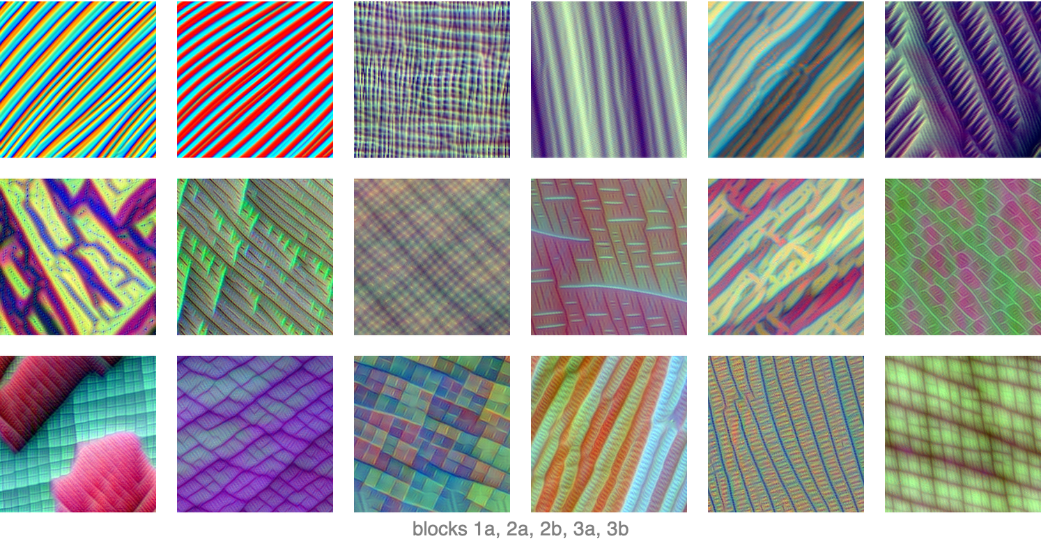
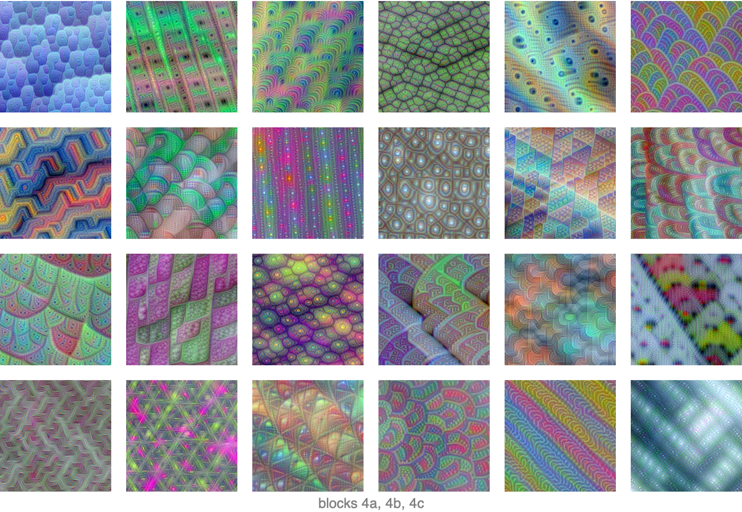
Again, the patterns are pretty simple, mainly lines in one or more directions. This shows that these kernels are detecting simple features. Interestingly, the bottom-left image shows two kinds of patterns overlapping, which means that this kernel (from block 3a) detects two kinds of things. Let’s now look at what activates channels in blocks 4a, 4b, and 4c:
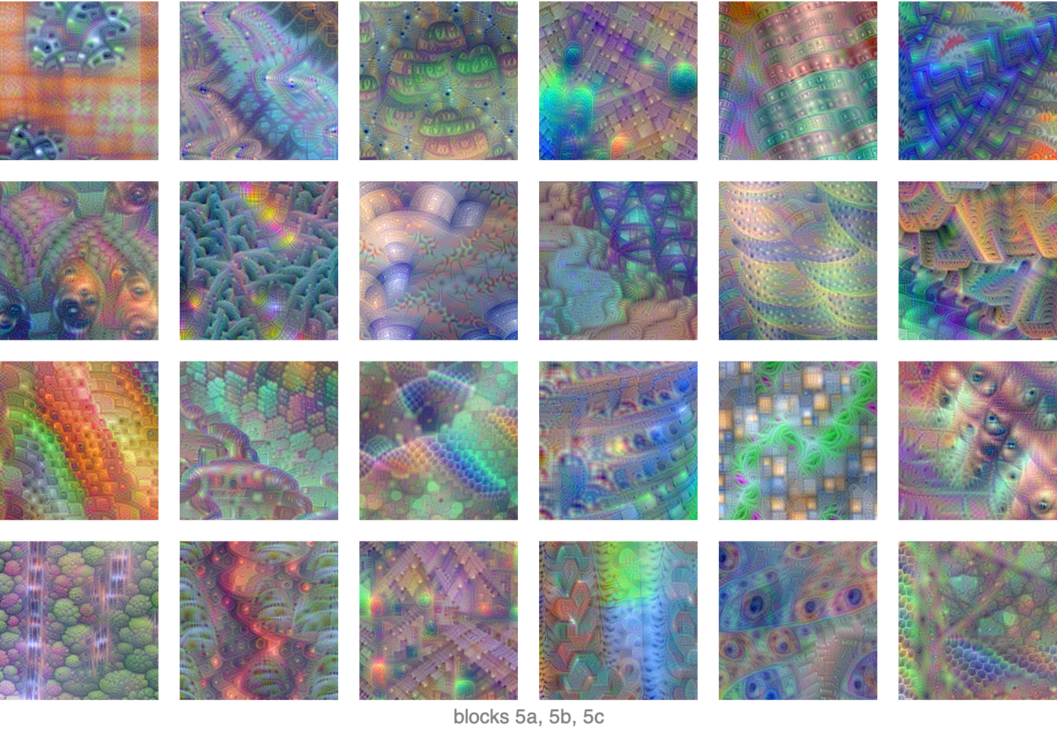
We can see that the patterns are more complex. Some kernels seem to detect curved lines and circles while others seem to detect textures. We cannot see any object-like shapes yet. These are mid-level detectors in terms of complexity. Let’s now look at what activates channels in blocks 5a, 5b, and 5c:
The images appear more complex and less repetitive. We can see more interesting patterns and even shapes that look like object parts. Clearly, these layers are in charge of detecting higher-level concepts than previous layers. Finally, let’s look at what activates the channels in the final layers:
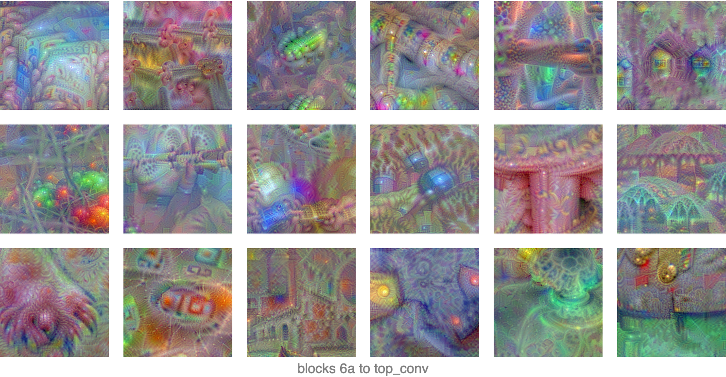
Now the repetitive patterns are almost completely gone; it’s like the optimization process is trying to generate something real. It is not easy to interpret what these images are supposed to be, but their diversity shows that these final layers are detecting complete objects or scenes.
Overall, we can see that this convolutional network is working in hierarchical fashion: first detecting simple shapes, then more complex shapes and textures, then object parts, and finally full objects and scenes. This is typically how convolutional networks, and deep neural networks in general, work. This staged detection process allows us to take advantage of the fact that the world is often hierarchical and compositional.
Other Convolutional Networks
Image classification is the most classic application of convolutional neural networks, but they can be used to solve other tasks as well.
A classic task tackled by convolutional neural networks is object detection, which means finding and classifying the objects present in an image, such as in this example:
This task is particularly important for self-driving vehicles. Here is a network to detect objects:
As we can see, this network has three outputs. One is returning the position of the bounding boxes, one is returning the confidence that there is an object in each box (the “objectness”), and one is returning class probabilities for the objects. Most of the weights in this network are in the first block, which is a rather classic convolutional network. One thing to notice though is that the spatial dimensions are only reduced to 1313 and not 11 as in classification. This makes sense because the network needs spatial information to predict where the objects are. A resolution of 1313 is detailed enough if objects are not too small.
Another classic task of convolutional networks is image segmentation, which means classifying each pixel according to the type of object they belong to. Here is a network for this task:
This network has been trained to segment biological cells on a substrate:
Let’s look at the architecture of this network:
We can see that blocks are connected in a main chain, which reduces and then increases the spatial dimensions. Then there are four skip connections that connect different parts of the chain. The graph displays as a U shape, which is why it is called a U-Net. The idea behind these connections is that, for the image segmentation task, the network needs to compute semantic information to detect the objects while also retaining precise spatial information to know the positions of the objects it detects. Instead of having the network remembering spatial information in its activations, the skip connections give the possibility for the network to copy previous activations. There is one skip connection at every scale, which allows for the placement of intermediary object parts, shapes, etc.
Convolution networks are not limited to images. Here is a network used to recognize speech:
Let’s use it on a recording:
Let’s now look at its architecture:
We can see that the first layers are convolutions. This is only true at the beginning of the network though; the following layers are recurrent ones (see the section Recurrent Networks in this chapter). Some audio networks do use convolutions all the way, such as this network, to detect the pitch of a sound:
Convolutional networks are also used for text, but recurrent and transformer networks tend to be the most common architecture for this kind of data.
Recurrent Networks
Let’s now introduce recurrent neural networks (RNN), which are particularly interesting since they are closer to what one would expect of intelligent systems: they process information step by step while updating their “mental state.” Recurrent networks are heavily used, mostly to process sequential data such as text, audio, time series, or any other temporal data.
General Idea
Sequences are a special kind of data: their elements are similar in nature, the order of their elements matters more than the elements’ exact positions, and, importantly, their lengths vary. In principle, it is possible to use classic fixed-size data methods on sequences (see Chapter 9, Data Preprocessing), but it is usually better to use methods that are specifically designed for sequences.
We have seen that the Markov model method (see Chapter 10, Classic Supervised Learning Methods) is able to handle sequences directly. The issue with this method is that while processing a sequence, the model can only use information from the last five or six elements at most. This tiny memory prevents the model from extracting information resulting from the interaction of elements far apart. Convolution layers have a similar problem, which is solved by stacking several convolutions together. Recurrent neural networks offer a direct solution to transmit information along an entire sequence.
A recurrent network can be seen as a module processing sequences in a given direction while keeping and updating a state. This state allows it to remember things from the past of the sequence. Here is a classic representation of a recurrent layer:
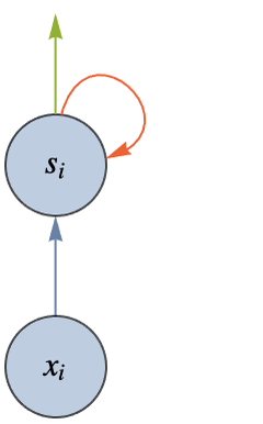
Here xi is the i th element of the sequence and si is the state of the network after processing this element. xi and si are typically numeric vectors. The self connection in red means that the state si is used to compute the next state si+1. This network looks quite different from what we have seen so far, but let’s say that the sequence to process it is of length 3. We can then unroll the recurrent network for this particular sequence:
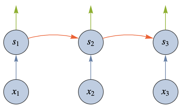
Now this looks more like a regular fixed-size network with the particularity that weights are shared since the same module is used along the sequence (a bit like a convolution but with a memory). In this case, the network has three outputs (the states computed), but it would have four outputs for a sequence of length 4 and so on.
In a recurrent network, the next state is always computed using the same function:
Computing all states is equivalent to the “fold” operation in functional programming:
Thanks to this architecture, the network can—in principle—remember things it processed earlier in the sequence and combine them with the rest of the sequence. In a sense, such behavior is closer to what animals/humans do since they continuously update their mental state according to their observations and previous mental states. Such networks are actually used to model agents behaving in an environment (such as in a reinforcement learning setting).
Recurrent neural networks can also be made “deeper” by stacking several of them together. Here is an unrolled recurrent network with two layers stacked on top of each other:
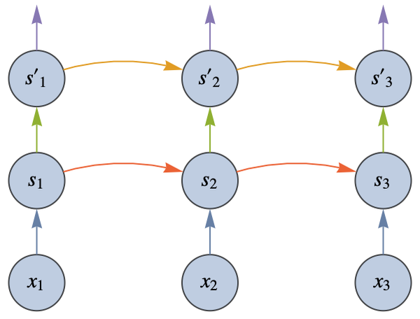
Like other deep networks, stacking several layers allows for the computation of more complex patterns. Such deep recurrent networks are very common.
Another variant is recurrent networks that read the sequence in both directions. These networks are called bidirectional recurrent networks. We could stack several layers that read in different directions, but the common approach is to use two regular recurrent networks that independently process the sequence in different directions and then join their results:
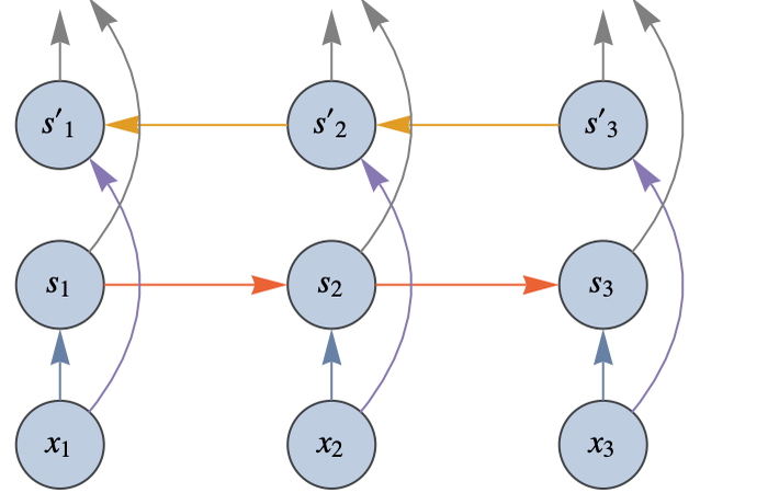
Bidirectional recurrent networks are usually better than unidirectional ones, but they cannot be used to generate sequences efficiently (see the Sequence Generation section in this chapter) or to model the behavior of an agent since they require knowledge of the future of the sequence, which does not exist yet.
We can train recurrent networks in the same way as any other network. The difference is that we need to unroll the network for each training sequence. Once unrolled, we can backpropagate the loss down to the parameters and obtain the gradient. This unrolling plus backpropagation is called backpropagation through time. Note that unrolled networks have different sizes, but we can still compute the gradient of the cost with respect to the parameters since it is a sum over individual training examples.
Recurrent neural networks have been the best method for text and generic sequence processing for a long time. They are still heavily used nowadays, but transformer networks are often the best method to process text (see the Transformer Networks section in this chapter). One issue that recurrent neural networks have is that they have trouble remembering long sequences. Another issue is that recurrent neural networks are fundamentally sequential and thus harder to parallelize in order to speed up the training phase.
Vanilla Recurrent Networks
Okay, let’s now construct an actual recurrent network. One of the simplest kinds is just using linear connections (that is, fully connected layers) to compute the state. Here is what such a vanilla recurrent network looks like for a sequence of three elements:

Here each element xi of the sequence is a vector of length 3 and each state si is a vector of length 2. We represented every connection like in a multilayer perceptron. You can see that each state vector si is computed both from the corresponding input xi and the previous state vector si-1. The connections here are using fully connected layers, so we can compute the next state vector in the following way:
Here Wx is the weight matrix applied to the input element, Ws is the weight matrix applied to the previous state, b is a bias term, and g is a nonlinearity. The same operation can also be performed by first joining the input element and the previous state to form a single fully connected layer. Let’s define this recurrent network. We can do it by first defining a core network:
Then we can wrap this core into a fold operator while indicating the recurrent connection:
Now we can use this recurrent network to process sequences. Here is the result for a sequence of two elements:
Here is the result after adding one more element:
We can also create this network in one step using a built-in layer:
Stacking several layers is done the same way as with any other kind of layer. Here is a chain of two recurrent layers:
Note that there is already a nonlinearity inside each recurrent layer, which is why we did not add any. Such a chain of recurrent layers is also a recurrent network. Let’s “unfold” this network to recover its core:
We can see that this recurrent network has two states, but we could merge them to form a unique state if we wanted to.
One problem that these vanilla recurrent networks have is that they are hard to train. Indeed, recurrent networks are as long as the sequence they process, and gradients tend to get very small or very large for such highly composed functions. One way to intuitively understand this is to realize that, during backpropagation, the gradient is multiplied by a matrix at each backpropagation step. This is a bit like multiplying many random numbers: if the numbers are typically smaller than 1, their product goes to 0 quickly:
If the numbers are typically larger than 1, their product goes to infinity:
This phenomenon is called the vanishing and exploding gradient problem and is also present for regular deep neural networks when they do not have the appropriate architecture, initialization, or normalization of the activations.
Besides optimization problems, such vanilla recurrent networks are also not very good at remembering things for a long time. Overall, their inductive bias is not the best. For all these reasons, vanilla recurrent networks are not used much anymore. Recurrent networks using gating mechanisms obtain much better performance.
Long Short-Term Memory Networks
The long short-term memory (LSTM) architecture had been introduced in the 90s (but it only became commonplace quite later) to overcome the shortcomings of vanilla recurrent networks. This architecture played an important role in the deep learning revolution of the 2010s; it has been used in many commercial applications, such as for speech recognition or text translation. LSTMs had been pretty much unrivaled for sequence processing until the end of the 2010s and the introduction of transformer networks.
Here is the core network of the LSTM architecture:
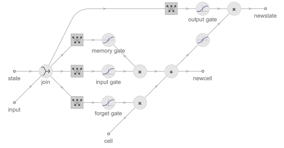
As we can see, it is a bit more complicated than for vanilla recurrent networks, but it all makes sense…. Every edge corresponds to a vector of numeric values. The first thing to notice is that there are two types of state vectors: the regular state, which is also the output, and a cell state, which is only there to transmit information to the next computation step. Then we can see four linear layers followed by nonlinearities, which all compute something from the input element and the state. These are the gates of the LSTM because their output is multiplied with another vector, hence, modulating the value of this vector. These gating mechanisms are at the core of the LSTM architecture.
Let’s focus on the three bottom gates, which are used to update the cell state. The forget gate (at the bottom) computes a vector of numbers between 0 and 1, which is then multiplied with the cell state. This means this gate has the ability to erase some values of the cell state. The input gate (above the forget gate) also computes numbers between 0 and 1, which are then multiplied with the memory gate (above the input gate), and the result is added to the cell state. This means that the memory gate is computing what should be added to the cell state and that the input gate decides if these numbers should indeed be added or not. The output gate (at the top) then decides which values of the cell state should be transmitted to the new state.
The LSTM architecture is particularly interesting because the cell state mimics actual computer memory: values are written or erased explicitly. This network looks more like a Turing machine than what we saw previously. Note that all these operations are continuous. This is unfortunately a requirement for neural networks because discrete operations (e.g. a true erasing using a step function) cannot be learned efficiently using gradient descent. LSTMs are much better at learning than vanilla recurrent networks, and they can sometimes remember things for hundreds of steps. This makes sense given that the cell state acts like classic memory. Another interpretation is that the cell state is a sort of skip connection, like in a residual block.
Let’s create an LSTM network that takes a sequence of vectors of length 3 as input and returns a sequence of vectors of length 2 as outputs:
The outputs are the states computed at every step. By definition, the cell state has the same size as the regular state:
Let’s apply this LSTM to a sequence:
As with vanilla recurrent networks, we could also stack such layers to form a deeper network or use a bidirectional version of this layer.
Variations of this architecture have been developed, such as the gated recurrent unit (GRU) architecture (in 2014), which is a bit simpler than the LSTM architecture and obtains slightly better performance. On the research side, various extensions have been introduced to handle the network memory in a more long-term way (such as memory networks or neural Turing machines) but these extensions never really managed to take over the LSTM architecture. LSTM was the workhorse of sequence processing until the end of the 2010s and is still heavily used nowadays.
Sequence Classification
Let’s now use recurrent networks to train a text classifier. We will use the same topic classification dataset as we did in Chapter 3, Classification. We first create the training set from Wikipedia pages:
This dataset has about 700 sentences. Here is a random example from the training set:
Let’s now create a validation set:
Note that the training set and validation set are created from different Wikipedia pages. As a general rule, the validation set should be as different from the training set as possible to make sure that our model generalizes well. In this case, it would be even better to use a validation set coming from another data source.
Let’s now create a network that can classify text. First, we need to tokenize the text (see Chapter 9, Data Preprocessing). Given the small amount of data that we have, the best strategy here is to tokenize the sentences into words. Here is a preprocessor to do this:
Let’s now define the network:
The first layer is an embedding layer that transforms each word into a vector of size 100. These word representations will be learned during the training (this is equivalent to a one-hot encoding followed by a linear layer). The second layer is a dropout layer, which is there for regularization purposes. The third and most important layer is the LSTM layer, which returns vectors of size 100. To compute class probabilities, we need a fixed-size vector. To do so, we only use the last vector that the LSTM produces using the SequenceLastLayer function. Finally, we include a linear layer to change the vector size to the correct dimension (the number of classes) and a softmax to obtain probabilities. This is one of the simplest and most classic text classifiers that we can define using an LSTM layer.
Let’s train this network for 100 training rounds:
We can see that the error rates of both the training set and the validation set are decreasing and then plateauing. There is no sign of overfitting (the validation cost does not increase), and a quick hyperparameter search shows that this setting (a vector of size 100 and dropout rate of 95%) gives good results. This might be surprising given the high number of parameters in our network (about 4 million), but using large and regularized networks is often a good strategy to obtain good predictions. The downside is that these networks are bigger, slower to train, and slower to evaluate. Let’s try this network on an example:
This result is correct, and the training reports tell us that about 28% of the validation sentences are misclassified, which is better than a naive baseline (40% here) but not great since we obtained 22% errors on the same dataset in Chapter 3, Classification. This poor result is caused by a lack of data. Indeed, as with most other deep learning models, recurrent neural networks work best on large datasets. In our case, the dataset is tiny (700 sentences), which is why classic machine learning methods perform better.
Let’s now try to improve this result using transfer learning. The classic strategy is to used word embeddings (see Chapter 9, Data Preprocessing). In our case, let’s use the contextual word embeddings given by the BERT model:
We just need to apply this pretrained network to every sentence of the training set and validation set:
Then we need to define a network on top of these features:
Notice that the embedding layer is gone. We also reduced the output size of the LSTM a lot because it happens to work better in this case, which leads to a neural network that is quite a bit smaller. Let’s train this network:
This time the error is only about 10%, which outperforms all our previous classifiers. Let’s extract the trained network and join it with the preprocessing network:
We can now use the resulting network on sentences:
Sequence Generation
Let’s now apply recurrent networks to generate sequences. In the case of text, this task is known as language modeling. Let’s create an English-language model by learning from the following Wikipedia pages:
There are about 2000 sentences. Here is one of them:
Our goal is to create a model that can generate similar sentences.
The idea is to train an autoregressive model, which means a model that predicts the next element of a sequence given previous elements, like the Markov model that we saw in Chapter 10, Classic Supervised Learning Methods. From this model, we can generate sequences element by element. We could train such a language model like a usual classifier, meaning with input-output pairs such as:
The training of such a classifier would be rather slow though because the network only learns to predict one element per sequence. A faster way to train an autoregressive model is use the teacher forcing technique, which means setting up a training network that predicts each next element in the sequence:
We can then extract a classifier from this training network. Importantly, the training network should only have access to previous elements when making a prediction, which is easy to do with a unidirectional recurrent network.
Okay, let’s create such a training network. We choose to generate the sentences character by character. Here is our vocabulary:
Let’s now define a network that predicts every possible next element of the sequence:
This network processes a sequence of vectors using gated recurrent layers, which is an alternative to LSTMs. The architecture of this network is similar to a recurrent classifier except that the last linear and softmax layers are applied independently to each vector of the sequence rather than only to the last vector. Let’s now define the training network:
Inside this network, the next characters are predicted and compared to the real next characters using a cross-entropy loss. Let’s train this network:
The validation error seems to plateau around 38%, which is not that surprising given the inherent uncertainty of text generation. The validation cost is 1.35, which is the mean cross-entropy per character. This measure is often reported in base 2:
This means that we could use this model to compress similar texts (generated from the same distribution) at a rate of 1.95 bits per character. Another classic way to report this measure is to compute the perplexity, which is the exponential of the mean cross-entropy per character:
In order to generate text from this trained network, we need to do a bit of surgery. First, we extract the trained network that predicts every character:
Then we need to convert the last linear and softmax layers to only act on the last vector of the sequence:
Finally, we need to add proper preprocessing and post-processing to handle strings:
We now have a network that should be able to generate a plausible next character given a string. Let’s see what it predicts after the characters “Th”:
So far so good. Let’s now generate text by feeding the predictions back into the network iteratively:
As we can see, the text repeats itself. This is because the network always predicts the most likely character. To generate random text according to this learned distribution, we need to sample each character from their predicted probabilities. Let’s perform such a sampling until a period is generated:
We now have a random “English” sentence. This way of generating sequences is not efficient though because the network keeps on reprocessing the same text. A better way is to extract the states of the recurrent layers after each iteration and to reuse them for the next iteration. We could do this by first unfolding the recurrent network to obtain its core network:
Then we can create a program that reinjects in the core network both the predicted character and the states at each iteration. A simpler solution is to use a specific tool that does exactly what we need by keeping the states of the recurrent network in memory:
The generation speed is now proportional to the length of the sentence.
As we can see, the English of these sentences is not great, to say the least. Learning to generate plausible text is a difficult task that requires more data and bigger models. Nowadays, the best language models are using the transformer architecture (see the Transformer Networks section in this chapter) and are trained on datasets containing hundreds of billions of tokens.
Sequence-to-Sequence
Recurrent networks can process and generate sequences. By combining both approaches, we can use recurrent networks to convert a sequence into another sequence. This is a sequence-to-sequence task, also called seq2seq, and its most typical applications are text translation and speech recognition.
To introduce this task, let’s create a model to perform symbolic integration, which means finding the primitive of a mathematical expression. For example, the primitive of x2 is ![]() :
:
The Integrate function is currently implemented with traditional programming, and as of 2020, it is unclear if machine learning can help with this task. Let’s train a simple machine learning model on this task.
Ideally, we should use real-world data, but to make things simpler, we are going to generate a synthetic dataset. Here is a function to generate random expressions:
The idea is to add, multiply, or divide simple expressions together (x, Sin(x), Cos(x), ![]() , etc.). Here is a random expression:
, etc.). Here is a random expression:
Integrating is hard, but differentiating (the inverse operation) is easy, so we generate a dataset by differentiating random expressions to obtain the inputs, and the outputs are the original expressions. Let’s generate input-output pairs:
Because of duplicates, we generated about 30000 pairs, which we separate into a training set and a test set:
Here are the first five training examples:
We need to encode these expressions so that our neural network can read and generate them. A natural solution is to use a tree structure:
Some neural networks can process trees (and even graphs), but they are not easy to implement with current tools. To make things simpler, we represent this tree as a sequence in a depth-first fashion:
From this sequence, we can reconstruct the original expression if we want to:
Since we are going to generate the outputs element by element, we need to know when to stop. To do this, we add an end-of-sequence token to each output. We also add a start-of-sequence token to let the network learn the proper initialization for the recurrent state. Let’s encode our training data and add these tokens:
Here is the first training example with its tokens colorized:
And here are all possible tokens:
The data is now ready. Let’s implement an appropriate network.
The typical way to convert a sequence into another sequence is to decompose the network into two parts. First, an encoder network processes the input sequence and transforms it into a numeric representation of some kind. Then a decoder network reads this representation to generate the predicted output sequence. Here is our encoder network:
As you can see, this network is similar to a classifier: there is an embedding layer and recurrent layers and it returns the last vector generated:
This last vector is our internal representation for the input, which is often called a latent representation or sometimes a thought vector. This is similar to the vector at the bottleneck of an autoencoder (see Chapter 7, Dimensionality Reduction). Using a vector as an internal representation is not a requirement. It is also possible to use the entire sequence of vectors (see the Transformer Networks section in this chapter).
Let’s now implement the decoder part. This is a generating network, similar to a language model, except that it needs to be conditioned on the representation computed by the encoder. To do this, we set the initial state of the recurrent network with the output of the encoder. Here is the decoder:
The "Sequence" port corresponds to the elements generated so far, and the "Vector" port corresponds to the output of the encoder. This network is set up to be trained using the teacher forcing strategy, so we will need to do a bit of surgery after training to obtain the “true” decoder.
We can now join these two networks into a training network that includes a loss function:
Notice how the decoding part is identical to the training network that we created for sequence generation.
Let’s train this network on our data:
The validation cost is decreasing and plateaus after about 20 training rounds. The final error is about 0.6%, but we should remember that this is the error rate when generating a single element, so the error rate of the full output sequence should be quite a bit higher. To test this, let’s extract the inference network from the training network. We first need to extract the encoder network:
This part does not need surgery; we can readily use it to encode input sequences into vectors. Let’s now extract the decoder and perform the necessary surgery:
Here we converted the original decoder to only return the last vector and added proper preprocessing and post-processing to handle the vocabulary elements.
We now need to join the encoder and decoder somehow. Since we need to reinject the predictions made by the decoder, we cannot create a single seq2seq network. We have to write a small function around the encoder and decoder to make predictions:
At first, the encoder is used to obtain the vector. Then the decoder generates elements one by one until the end-of-sequence token is generated. Here we greedily pick the most likely element given past ones. This procedure does not generate the most likely sequence given the input though. To obtain the most likely sequence, we should perform an optimization procedure, the most common one being beam search, which, in a nutshell, keeps a bag of k (the beam size) most likely sequences during the decoding. To keep things simple, we keep this greedy solution (which is equivalent to a beam search with k=1). Let’s try the predicted primitive on a simple expression:
Not surprisingly, it is correct. Let’s now try it on the first five test examples:
These seem correct as well. Let’s see how many predictions are correct on 1000 test examples. Since the same mathematical formula can be written in different ways, we perform a numeric test:
We see that 92.4% of the test examples are correctly predicted, which seems rather high given how naive this approach is. To stress test this model further, let’s try it on examples that are out-of-distribution (a.k.a. out-of-domain), which means they are sampled from a different distribution than the one we used to generate the training set:
As you can see, the result is wrong, and it does not take much to find the weak spots of this network. This is a reminder of how brittle machine learning models can be for some tasks. One solution to improve the robustness here would be to train on data that is much more diverse. As of 2020, traditional algorithms are still the best solution for this task, which is not surprising since it requires symbolic manipulation, which is not the domain of predilection of machine learning models. Here is another example that does not work:
In this case, the predicted expression is not even valid because a bracket is missing. Indeed, because we decode the expression as a sequence, we are not guaranteed to obtain a valid expression. This is particularly problematic for long sequences since recurrent networks cannot remember things for a long time, so they might forget that a bracket had been open in the beginning of the expression. One solution is to encode and process expression trees directly. Another solution is to use models that are better at remembering things for a long time, such as the transformer architecture.
Transformer Networks
Let’s now look at our final neural network architecture called transformer networks or just transformers. This architecture had been introduced in 2017 and led to important progress in the field of natural language processing, quite like what happened in the field of computer vision in the early 2010s. Nowadays, transformers are heavily used, mostly as pre-trained networks, and they obtain the best performance on just about every classic natural language processing task.
Attention
At the heart of the transformer architecture is the concept of attention. In psychology, attention is the process of focusing on specific information while ignoring other information, such as looking at a specific object while ignoring other things in our visual field. This allows us to reduce the cognitive load necessary to solve a task. Such a mechanism can also be used in neural networks. Of course, this strategy is only beneficial if semantic information is localized, which is the case for images because they contain localized objects or for text because it contains words.
How can we create an attention mechanism for neural networks? Let’s say that the input of the network is a list of vectors:
Each of these vectors represents a particular part of the input, such as a word (they would then be word embeddings) or a part of an image. Attention means focusing on one of these vectors, which really means selecting this vector. In neural networks, attention could just as well be called “selection.” A straightforward way to select a vector is to use its position:
This is like retrieving a value in classic computer memory. An alternative way is to find the nearest vector to a query vector:
This is closer to the associative array data structure or to the content-addressable memory of some computers.
In principle, we could implement a network that uses such a selection operation. The network would first compute a position (“3” here) or a query vector, and then select the target vector. This is called a hard-attention mechanism. The problem with hard attention is that it is a non-continuous operation and that non-continuous operations prevent gradient descent optimization from working well. Other optimization procedures could be used, but they are slower than gradient descent. The solution is to use a soft-attention mechanism.
The idea of soft attention is to compute a weighted sum over input parts such as:
Mathematically this is:
The weights {0.1,0.05,0.8,0.05} are called attention weights or attention scores. Here the vector at position 3 is given the highest score (0.8) while others have scores below 0.1. The output is, therefore, close to the third vector but not exactly equal; this is a soft selection. These scores are computed by the network, and when they are normalized, they form an attention distribution.
Okay, so how does the network compute these attention scores? The idea is to use a content-addressable approach. Each input vector is compared to a query vector, and a similarity score is computed. The most simple way to compare vectors is to use their dot product (but we could use other similarities as well):
These scores are then passed through a softmax to obtain the attention distribution:
In this case, most of the attention is on the third vector. We can now compute the final output of this soft selection:
We can see that the third vector is (softly) selected. Here is this procedure as a neural network:
The last two operations can also be computed more efficiently using matrix multiplication:
This soft-selection procedure is the most common kind of attention.
In the previous example, the input sequence is used to obtain an output but also to compute the attention scores. In some cases, we want to dissociate these two roles by using a set of keys and a set of values instead of a unique set of inputs. The key vectors are compared to the query, and the output is a weighted average of the values. Here is an example:
Note that the values can now be of a different type than the keys. Modern attention is usually defined in this way. Here is this attention operation summarized into a unique attention layer:
We used a dot product as a similarity here. Dot product is the most common similarity choice because of its simplicity and computation speed, but in some cases, another similarity might work better.
Note that there is a relation between gating mechanisms (as in the LSTM architecture) and attention mechanisms because they both use multiplication to select some elements. The main difference is that attention returns a unique element (through a softmax and a sum) while gating mechanisms are just modulating the value of the elements.
This is basically what attention mechanisms are: a simple way to implement a selection mechanism for neural networks. Attention was introduced in 2015 and is now considered a fundamental operation that neural networks can make use of. As of 2020, attention is mostly used in natural language processing, but it is likely to spread to other areas.
Attention in Recurrent Networks
Attention mechanisms were originally used in recurrent neural networks, and in particular to improve the performance of recurrent decoders. A classic example is text translation. For example, let’s look at this English-to-French translation example:
This is a seq2seq task that can be tackled using an encoder and decoder recurrent network (see the Recurrent Networks section in this chapter). A recurrent encoder would produce one numeric vector per token (which are words here), such as:
Previously, we used the last vector to feed the decoding process. When attention is used, we would use the entire sequence of vectors. At each decoding step, the decoder uses its current state as a query to attend over the vectors produced by the encoder. Here is an illustration showing the sequence of operation for one decoding step:
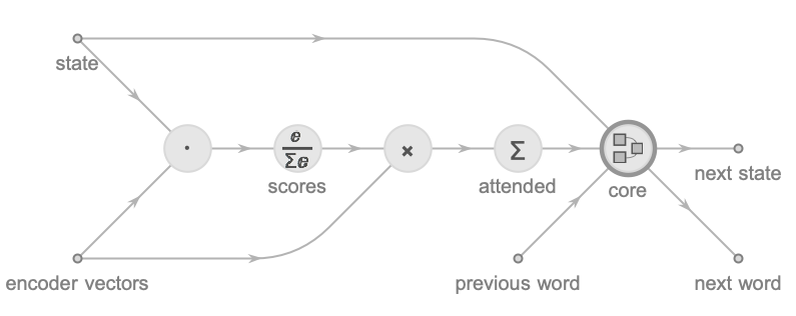
You can see that the decoder compares its current state with every encoder vector in order to choose which one should be used to generate the next word. The network learns to focus on what’s important at each step. This mechanism makes sense here since there is a direct correspondence between words: “chat” is the translation of “cat,” “tapis” is the translation of “mat,” and so on. Here is an example of attention scores obtained by such a network on a translation task:
We can see that at each step, the decoder chose to attend over one or a few words that are relevant. This is similar to how humans would translate. This technique led to important progress in text translation.
Attention can also be used in computer vision. Here is an example of the task of image captioning:
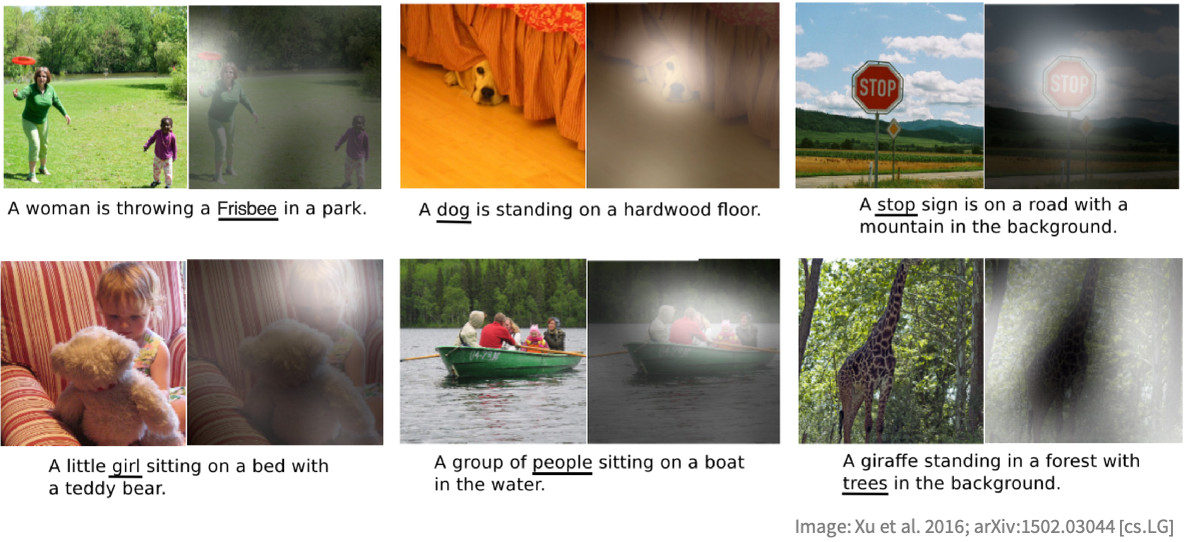
The procedure is the same as in the translation example. A convolutional neural network processes the input image into a list of vectors with each of these vectors representing information located in a part of the image. Then a recurrent network generates the caption one word at a time. At each step, the decoder network decides which vector (that is, which part of the image) it should focus on. In the first image, we can see that the decoder focused on the Frisbee when generating the word “Frisbee,” which makes sense. In this case, attention can improve performance, but it is also useful to interpret what the network does.
Another way to include attention in a recurrent network is to attend over previous elements of a sequence. This is called self-attention or intra-attention. Here is an example in which a unidirectional recurrent network processes a sentence word by word while attending over previous words:
The blue shading shows the attention scores when processing the words in red. We can see that when processing the word “run,” the network attends over previous words but also “FBI,” which is probably relevant to disambiguate the meaning of “run.” Here the recurrent network uses both its current state and the attended vector to compute its next state. This self-attention mechanism can be used in encoders as shown here but also in decoders to give the possibility of looking back at the token generated so far. One advantage of using self-attention is that it is possible to look back farther in the past in order to get the necessary information. This is a solution to the memory problem of recurrent networks.
Attention has been pretty successful at improving performance of recurrent networks, and the combination of recurrence plus attention is likely to play a role in the future of natural language processing and machine learning in general. Nevertheless, state-of-the-art models in natural language processing are not using recurrent networks anymore but the transformer architecture, which makes for more extensive use of these attention mechanisms.
Bidirectional Transformer
Let’s start by introducing the bidirectional transformer architecture, which is used to process sequences. This architecture could, for example, be used to create a text classifier, a text feature extractor, or the encoder of a translation model.
The hallmark of transformers is that they use self-attention. We saw that recurrent networks could use self-attention to improve their performance, but there is then a redundancy: the information is transmitted both by the recurrent state and the attended vectors. The idea of transformer networks is to drop the recurrence entirely and purely rely on self-attention. This is well summarized by the title of the paper that introduced this architecture, “Attention Is All You Need.” This drastic idea happens to work quite well in practice, at least for sequential data.
Before diving into the details of the transformer architecture, let’s try to understand the consequences of using self-attention in terms of information processing. If the task is to process a sequence (as opposed to generate a sequence), self-attention means that every input vector attends over every input vector. Here is an illustration of how the information flows in such a self-attention layer:
The input is a set of vectors (the initial word embeddings in this case), and the output is another set of vectors, exactly like in a recurrent layer, but there is no recurrence relation between outputs here. Instead, the output vectors are computed from all input vectors and in both directions. This is reminiscent of fully connected networks but is actually quite different because attention is used here, which discourages complex overfitting-prone relations to be modeled (also, fully connected networks could not be implemented for sequences). Here the input vector corresponding to the word “ran” is compared to every input vector in order to decide which one(s) should be used to compute the next representation of “ran.” Such connectivity allows for the easy transfer of information from every part of the input to every other part. As a comparison, let’s look at the connectivity of a convolution layer:

In this case, information only flows from neighbor to neighbor. This poses problems if distant words happen to have a strong interaction. For example, in the sentence “The dog ran very fast over the hill because it was scared,” the word “it” refers to the word “dog.” In order to connect these two words, we would need several convolution layers. Let’s now look at the connectivity of a recurrent layer:

Here the information flows from the beginning to the end of the sequence, but it can only flow indirectly through the recurrent state. Such an architecture is not ideal for handling distant interactions either. Another problem of this recurrent architecture is that the processing is sequential, which means that we cannot compute all output vectors in parallel. When training a network on a CPU, this is not much of an issue, but when training on hardware such as GPUs or other highly parallel systems, this can be a constraint.
Thanks to their connectivity, transformers can quickly transfer information between elements of the input. Unfortunately, this also implies that the processing time scales quadratically with the length of the sequence because every element needs to be compared with every element. In contrast, the processing time of convolution and recurrent layers is only linear in the length of the sequence. This means that for long sequences, transformers can be much slower than convolution and recurrent networks. On the other hand, transformers need fewer layers than convolution networks, and they can be parallelized better than recurrent networks. This means that for some tasks (such as translating sentences) and some hardware (such as GPUs), transformers can end up being quite a bit faster to train, which makes it possible to use larger training sets and, thus, to obtain better models.
Let’s now dive into the transformer architecture in more detail. To do so, we use the classic BERT transformer model:
This network processes text and transforms every word (or subword) into a vector of size 768, which can then be used for a subsequent task (see Chapter 9, Data Preprocessing):
The first part of this network is embedding tokens into vectors. The original version of this embedding part is unnecessarily complex (it is made to handle two consecutive sentences). Here is a simplified version of it:
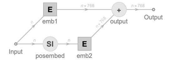
One branch embeds tokens (words or subwords) and the other one adds information about the position of each token:
This is important because the information about the position of each input is lost when using the transformer architecture. Let’s now look at the second part of the network:
This is a chain of 12 identical blocks, each of them taking n vectors of size 768 as input and outputting n vectors of size 768. Let’s look at one of these blocks:
Every edge corresponds to a sequence flowing into this network. We can see many linear layers wrapped by map operators (![]() ), which means that the linear layers are applied independently to each element of the sequence. All the learnable parameters of the transformer architecture are in these linear layers. There are two residual blocks here. The second block is simply a multilayer perceptron that is applied to each vector independently, so there is nothing really new here. The more interesting part is the first residual block, which contains the attention mechanism and is the core of the transformer architecture. Let’s analyze this block in more detail:
), which means that the linear layers are applied independently to each element of the sequence. All the learnable parameters of the transformer architecture are in these linear layers. There are two residual blocks here. The second block is simply a multilayer perceptron that is applied to each vector independently, so there is nothing really new here. The more interesting part is the first residual block, which contains the attention mechanism and is the core of the transformer architecture. Let’s analyze this block in more detail:
In the middle, we can see the attention layer ![]() , which takes three inputs: the queries, the keys, and the values. These attention layers are the only layers in the network that allow different sequence elements to communicate with each other. Exactly as explained earlier, the queries are compared to the keys using a dot product to compute attention scores, which are then used to select the relevant values. Since this is a self-attention procedure, queries, keys, and values are all coming from the same input (which is a sequence of vectors), but we can see that they are transformed by different linear operations before the attention layer. These transformations allow the network to come up with an appropriate representation for all of them. One important thing to notice is that for each element of the sequence, the linear layers create 12 different vectors of size 64, which means 12 queries, 12 keys, and 12 values for each element. Then, the attention layer performs 12 attention operations, which are independent from each other. The 12 resulting vectors are then concatenated into a single result and then processed by a linear layer. This is called a multi-head attention mechanism. Here is the original illustration of the multi-head attention from the paper that introduces transformers:
, which takes three inputs: the queries, the keys, and the values. These attention layers are the only layers in the network that allow different sequence elements to communicate with each other. Exactly as explained earlier, the queries are compared to the keys using a dot product to compute attention scores, which are then used to select the relevant values. Since this is a self-attention procedure, queries, keys, and values are all coming from the same input (which is a sequence of vectors), but we can see that they are transformed by different linear operations before the attention layer. These transformations allow the network to come up with an appropriate representation for all of them. One important thing to notice is that for each element of the sequence, the linear layers create 12 different vectors of size 64, which means 12 queries, 12 keys, and 12 values for each element. Then, the attention layer performs 12 attention operations, which are independent from each other. The 12 resulting vectors are then concatenated into a single result and then processed by a linear layer. This is called a multi-head attention mechanism. Here is the original illustration of the multi-head attention from the paper that introduces transformers:
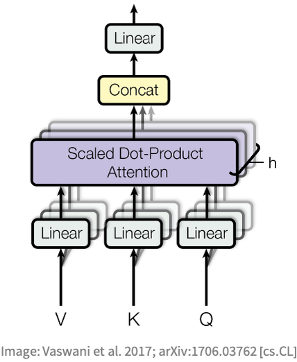
The advantage of multi-head attention is that each attention head can specialize in performing a specific operation. For example, when processing a verb (such as “ran” in “the dog ran very fast”), one attention head’s job might be to find the subject (“the dog” here) while another attention head’s job might be to figure out the related adjective (“fast”). We can think of these attention heads as different feature detectors, like the kernels of a convolution layer.
And that is how a bidirectional transformer works. Such a network can be used to process any sequence, which means any kind of data since we can convert anything into a sequence. The most important success of this transformer architecture so far has been to allow the training of large text-processing networks, such as BERT, which are used to perform transfer learning procedures for all kinds of applications. In 2020, it has also been shown that this architecture can rival convolutional neural networks for image classification tasks by using a vision transformer (ViT ) architecture, which is very close to the vanilla transformer architecture presented here.
Unidirectional Transformer
Let’s now introduce the unidirectional transformer architecture, which is a transformer architecture used to generate sequences.
Here is the connectivity of the bidirectional transformer described previously:

Such a transformer can be used to process sequences, create classifiers, and so on. In principle, we could also use it to generate sequences by simply training a classifier to predict the next element given past elements. The problem is that this strategy would be inefficient since we would need to reprocess the entire sequence from scratch at each element generation step. A smarter strategy is to design a sequence generator that only transmits information from the past to the future, such as:

Here the last vector would be used to predict the word after “fast.” With this architecture, we would only need to compute the representation for the new word and keep previous representations unchanged:
This allows for the efficient generation of sequences and the training of the sequence generator in a teacher forcing setting, which means predicting every next element of the sequence at once during the training. This type of unidirectional self-attention is also called masked self-attention because a mask is used to set all the backward connections to zero. Note that this unidirectional model can be seen as a kind of recurrent network for which the state is the sequence of past inputs (which means a variable-length state).
Besides using a masked self-attention, unidirectional transformers are in every point similar to bidirectional transformers. Here is GPT-2, a classic unidirectional transformer that has been trained to model English text:
The architecture is about the same as for BERT but the end of the network is different. We can see that a linear layer is applied to the last vector, which is then passed through a softmax to predict the probabilities for the next token. Like any other language model, we can use this network by giving it a sequence to obtain the most likely next word:
We can also obtain a random next word conditioned on previous words:
To generate a long string efficiently, we would need to do some surgery in order to return and reuse the representations computed previously by unfolding the network (see the next section).
Sequence-to-Sequence
Since transformers can process and generate sequences, we can use them to perform sequence-to-sequence tasks, such as text translation.
As for recurrent networks, the idea is to connect an encoder and a decoder network. The encoder can be bidirectional and the decoder has to be unidirectional for performance reasons. Here is the usual architecture to do this, as illustrated in the original transformer paper:
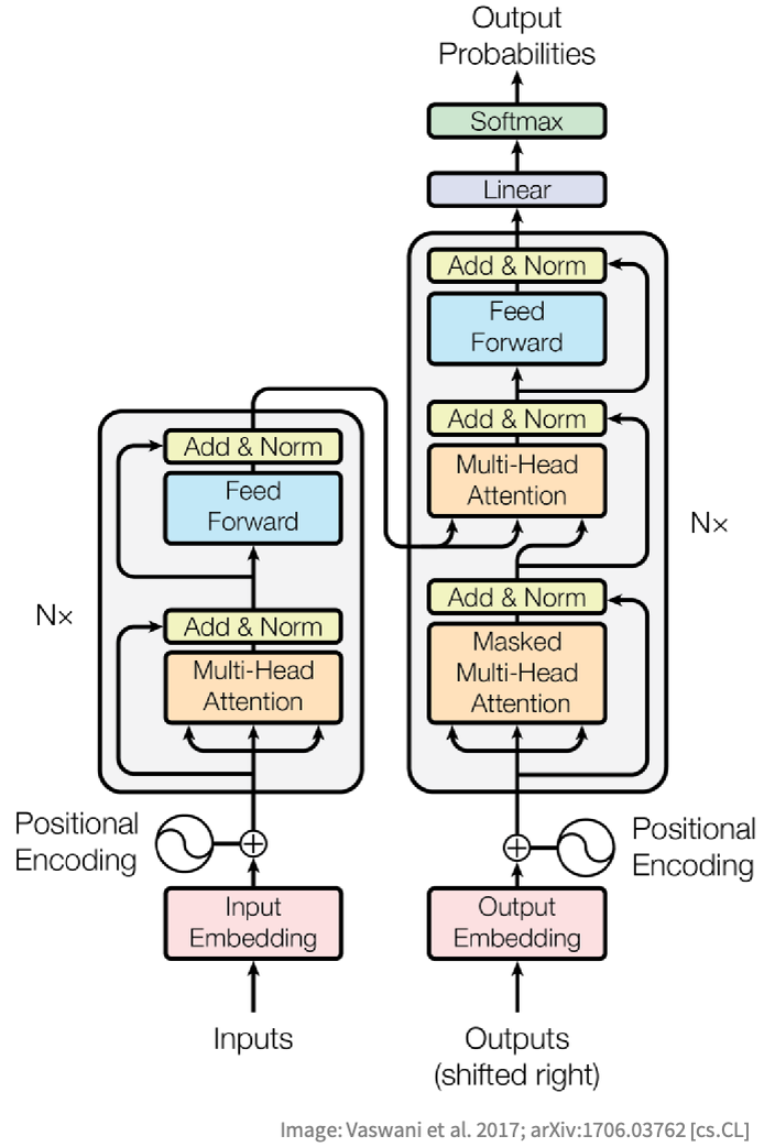
The encoder (on the left) is a classic bidirectional transformer that processes the input sequence. The decoder (on the right) is a bit more complex. Each block is first composed of a unidirectional self-attention that processes the output sequence. The result of this first attention procedure is used as a query to attend over the encoder output using another attention procedure (bidirectional this time). Note that there is a residual connection around this bidirectional attention procedure, so we can interpret this step as choosing which encoder output should be used in order to modify the current decoder representations.
To understand this architecture better, let’s use it on the symbolic integration task from the Recurrent Networks section in this chapter:
We use embeddings of size 128 with four heads and vectors of size 32 for the keys, queries, and values:
First, we need something to embed the sequences into vectors and add positional information:
Let’s now implement an encoder block:
From this, we can create the complete encoder (we use only use two blocks to train faster):
Let’s now implement a decoder block and visualize its connectivity graph:
This block has two inputs. The first one corresponds to the sequence generated and the second one corresponds to the encoder outputs. Let’s combine two decoder blocks and the embedding to form the complete decoder:
We can see how the decoder output is injected in each block. Finally, we need to create a training net, exactly as we did for recurrent networks:
We can now train this network on the symbolic integration problem:
The per-token error obtained is about 0.9%, which is a bit worse than what we obtained with recurrent networks (about 0.6%). We can see that the learning curve is still making progress though; we would gain from more training here. Also, validation and training costs are the same, so we would most likely gain from using a larger network. Note that this network has been quite a bit slower to train than the recurrent network (5 hours vs. 30 minutes). One reason for this is that we trained on a CPU and not a GPU. GPUs are better at taking advantage of the parallelization possibilities of transformers.
To use this network, we have to do the same procedure that we did in the recurrent case. We first need to extract the encoder:
Then we need to extract the decoder and perform some surgery on it to predict only the next element:
We now have to create a program to generate elements until the end-of-sequence token is generated (the same program as the one used for recurrent networks):
Let’s use this network on a simple example:
This network behaves quite similarly to the recurrent one. It works well on test data but very poorly on out-of-domain data, which makes it unusable in practice. Using a much more diverse dataset would be the first step to making it useful.
Note that in our integrate function, we naively reprocess the entire sequence for each prediction. To be more effective, we should perform an additional surgery to be able to extract and reinject the intermediate representations of the decoder. This can be done by extracting the core network of the decoder as we would do for a recurrent network:
This module can be used to obtain the next token and next representations from past representations and from the last token generated. In a sense, this decoder is like a recurrent network, but the state consists of all the past representations instead of a fixed-size vector in recurrent networks.
Sequence-to-sequence tasks are often tackled using the transformer architecture. Text translation is one of them. As we have seen in this example, transformers are not silver bullets though, and recurrent networks are still useful. Recurrent networks and transformers make different assumptions, which means an architecture can outperform the other depending on the application. As a rule of thumb, transformers are better when you can train on a powerful GPU-like machine, when there are long-range dependencies that recurrent networks have a hard time capturing, and when sequences are not too long either since the processing time is quadratic in the sequence length. As of the early 2020s, the transformer architecture is still in its infancy, so it is likely that improvements will be made to improve it further.
| From neurons to networks | |
| ■ | Neural networks are parametric models composed of layers processing numeric arrays. |
| ■ | Neural networks are mostly composed of linear operations and simple nonlinearities. |
| ■ | Deep learning means learning with a neural network that has many layers. |
| ■ | Deep learning methods are typically used on datasets that have many variables and many examples. |
| ■ | Deep learning methods are good for modeling human perception and intuitive tasks. |
| ■ | There exist several network architectures that can be used to solve different tasks. |
| How neural networks learn | |
| ■ | The parameters/weights of a neural network are learned by minimizing a cost function. |
| ■ | Stochastic gradient descent is used to perform the minimization. |
| ■ | Backpropagation is used to compute the gradient of the cost with respect to the parameters. |
| ■ | Backpropagation computes the gradient about as fast as running the network. |
| Convolutional networks | |
| ■ | Convolutional networks are networks using convolutions. |
| ■ | A (neural) convolution is a linear operation acting on a moving window. |
| ■ | Convolution layers are using several convolution kernels, each one of them detecting a specific feature. |
| ■ | A convolutional network can be seen as a sparse multilayer perceptron with weight sharing. |
| ■ | Convolutional networks are mostly used to process images. |
| Recurrent networks | |
| ■ | Recurrent networks are designed to process or generate sequences. |
| ■ | Recurrent networks process sequences element by element while keeping an internal state. |
| ■ | The internal state of a recurrent network acts as a memory. |
| ■ | LSTM is the most common recurrent architecture. |
| Transformer networks | |
| ■ | Transformers use self-attention to process or generate sequences. |
| ■ | Attention can be seen as a selection operation. |
| ■ | Self-attention means that every element of the sequence attends over every other element. |
| ■ | Transformers use several attention heads in parallel to compute features. |
| ■ | The time to process or generate a sequence using a transformer is quadratic in the length of the sequence. |
| ■ | Transformers led to impressive improvements in natural language processing. |
| neuron | brain cell that communicates with other neurons through electric signals in order to form a network able to compute things | |
| dendrites | branches from where the neuron receives its electric inputs | |
| axon | output branch of a neuron, transmits the signal to be sent to other neurons | |
| synapses | junctions connecting axons to dendrites | |
| spike | sharp electric signals fired by a neuron to be transmitted to other neurons | |
| artificial neuron artificial unit | simple processing system inspired by biological neurons, combines its input using a linear combination and applies a nonlinearity to the result | |
| activation function transfer function | nonlinear function used by artificial neurons | |
| weights | learnable parameters used to perform the linear part of an artificial neuron, sometimes used to mean all the parameters of a neural network | |
| bias | learnable parameter of an artificial neuron that is added after the linear transformation | |
| artificial neural network | machine learning model consisting of connected artificial neurons | |
| deep neural network | artificial neural network that has several layers | |
| deep learning | learning with deep neural networks | |
| layer | ensemble of artificial neurons that is used as a building block of a neural network; more generally, any parametrized module performing a simple computation from its inputs and sending its output to other layers | |
| hidden layer | layers that are neither the input nor the output (term mainly used in the context of multilayer perceptrons) | |
| block | ensemble of layers used as a building block to define networks | |
| activations | numeric values that are computed inside an artificial neural network | |
| neural architecture | class of neural networks sharing similar structures | |
| neural architecture search | automatic search of neural architecture and specific connectivity | |
| multilayer perceptron fully connected network feed-forward neural network | oldest neural architecture, chain of layers, every neuron of a given layer sends its output to every neuron of the next layer | |
| fully connected layer linear layer dense layer | layer of multilayer perceptrons, connects every input to every output | |
| matrix multiplication | generalization of the dot product for matrices, used by most network layers, can be efficiently performed by modern computers | |
| rectified linear unit (ReLU) | classic activation function, identity for positive activations and zero for negative ones | |
| scaled exponential linear unit (SELU) | variant of rectified linear unit used in self-normalizing neural networks | |
| self-normalizing neural network | multilayer perceptron variant that allows for the training of deep networks on structured data | |
| end-to-end learning | learning directly on raw data, without much preprocessing or manual feature extraction | |
| chain networks | chain of layers, each one connected to the next one in the chain | |
| graphical networks | set of layers connected according to a graph structure | |
| high-dimensional data | data for which examples are large/have many variables | |
| hierarchical data compositional data | spatial data for which local patterns form larger patterns and so on; image, text, and audio are examples of this kind of data | |
| symbol | categorical value representing a concept, an object, a relationship, etc.; text is made of symbols | |
| parallel computing | type of computation in which many calculations are carried out simultaneously, allowing for the use of many processing cores/units |
| gradient descent steepest descent | local optimization method that computes the gradient of the function-to-minimize in order to move along the steepest direction | |
| global minimum | a function has a global minimum at a given position if the function value at this position is the smallest | |
| local minimum | a function has a local minimum at a given position if the function value at this position is smaller than function values at surrounding positions | |
| local optimization method | optimization method that explores the function by doing small moves in the input space, might get stuck in local minima | |
| global optimization method | optimization method that seeks to find the global optimum of a function, any non-local optimization method | |
| basin of attraction | region of input space that leads to a given minimum of a function when using a local optimization method | |
| over-parametrization | having more model parameters than necessary to fit some data | |
| learning rate | hyperparameter controlling the step size of the gradient descent method, controls how fast we attempt to learn | |
| learning rate schedule | predefined plan for how to set learning rates during the optimization | |
| adaptive learning rate | when the learning rate automatically changes during the optimization | |
| gradient descent with momentum | extension of the gradient descent method that transfers some of the learning rate and step direction from one iteration to the next iteration, dynamic behaves like a ball rolling along the cost landscape | |
| Adam | classic adaptive learning rate method | |
| stochastic gradient descent method | variant of the gradient descent method where the gradient is computed using a subset of all training examples | |
| batch mini-batch | subset of training examples that is used to compute one gradient in the stochastic gradient descent method | |
| batch size | hyperparameter defining the number of examples present in a batch | |
| training round epoch | unit of time for the stochastic gradient descent learning process, corresponds to a complete cycle over all training examples | |
| derivative | rate of increase of a univariate function at a given point | |
| gradient | vector containing the derivatives of a multivariate function with respect to each variable, gives the steepest ascending direction | |
| Jacobian matrix | matrix of derivatives for a multivariate vector-valued function | |
| numerical differentiation finite difference method | method to compute the derivative of a function at a given position by comparing the value of the function at this position and at its surrounding positions | |
| symbolic differentiation | method to transform a symbolic expression of a function (a mathematical formula) into another symbolic expression that computes the derivative for any input | |
| chain rule | a way to efficiently compute the derivative of composite functions | |
| backpropagation | method to compute the derivative of the loss function with respect to the parameters, applies the chain rule to propagate the gradient of the loss from the last layers to the first layers | |
| forward pass | first part of the backpropagation procedure, evaluates the network and stores all its activations | |
| backward pass | second part of the backpropagation procedure, propagate the gradient from the the last layers to the first layers | |
| automatic differentiation | generalization of backpropagation for arbitrary programs | |
| directed acyclic graph | graph with directed edges that do not form cycles | |
| program trace | computational graph of a program for a specific execution, contains all instructions performed and all intermediate values that the program computed |
| convolutional neural network | neural network architecture that uses convolutions to process spatial data | |
| convolution | weighted moving average applied to an array of numeric values | |
| convolution kernel convolution filter | set of parameters defining a convolution | |
| kernel size | size of the kernel window | |
| stride | step size of the convolution | |
| zero-padding | padding an input with zeros to control the output size | |
| receptive field | size of the region in the input that produces a given activation of a neural network | |
| convolution layer | neural network layer that performs a convolution | |
| sparse connections | layer connections for which most input neurons are not connected to most output neurons | |
| local connections | sparse connections for which spatiality is preserved and for which input and output neurons are only connected if they are nearby | |
| weight sharing | constraining different connections to use the same weights, used to incorporate in the network some symmetry or invariance present in the data | |
| spatial locality assumption | assuming that in spatial data, there exists local patterns that are useful to understand the data | |
| translation invariance assumption shift invariance assumption space invariance assumption | assuming that in spatial data, the meaning of a local pattern does not depend on its position | |
| 1D convolutional network | convolutional network whose input has one spatial dimension, such as text or audio | |
| 2D convolutional network | convolutional network whose input has two spatial dimensions, such as images | |
| image channel | a slice of an image along its non-spatial dimension, usually representing the level of a given color; more generally, a slice along the non-spatial dimension of any array | |
| feature map | channel of some activation array of a neural network, represents the same feature computed at different locations of the input | |
| max-pooling layer | moving maximum, takes the largest value in each possible window of a given size, used to reduce the spatial dimensions of arrays | |
| dropout layer | regularization layer that randomly sets activations to zero | |
| batch normalization layer | layer that helps the training of neural networks by normalizing the activations across the examples of each batch | |
| skip connection | direct connection between two layers that were already connected through other layers, hence “skipping” those intermediate layers | |
| residual block | block with a skip connection that adds the input of the block back to the output of the block | |
| residual neural network (ResNet) | convolutional network composed of a chain of residual blocks | |
| squeeze-and-excitation block | block that uses a gating mechanism to modulate the activation of channels depending on the mean value of other channels, allows for a direct modeling of correlations between channels | |
| feature visualization | visualization of the input images that activate some parts of the network | |
| object detection | task of finding and classifying the objects present in an image | |
| image segmentation | task of classifying each pixel according to the type of object they belong to | |
| U-Net | a neural network that uses skip connections in such a way that the overall graph displays as a U shape, used for tasks such as image segmentation |
| recurrent neural networks | neural network architecture that processes or generates sequential data step by step while keeping an internal state | |
| state | values that a recurrent neural network keeps in memory to be used in the next processing/generating step | |
| unrolled network | recurrent network set up as a regular fixed-size network for a particular sequence length | |
| bidirectional recurrent network | recurrent network that processes sequences in both directions | |
| backpropagation through time | backpropagation applied to an unrolled recurrent network | |
| vanishing and exploding gradient | when the gradient of the loss becomes increasingly small or increasingly large as it propagates toward the first layers, occurs in recurrent or deep networks that are not properly architectured or initialized | |
| vanilla recurrent network | simplest recurrent architecture, uses fully connected layers to compute the next state | |
| long short-term memory (LSTM) network | standard recurrent architecture that uses gating mechanisms to improve the performance over vanilla recurrent networks | |
| gating mechanism | neural network mechanism that modulates activations by multiplying them by a number between 0 and 1 | |
| self-gating mechanism | gating mechanism for which the input is used to modulate itself | |
| cell state | extra state present in the LSTM architecture, used as a longer-term memory than the usual state | |
| gated recurrent unit (GRU) architecture | variant of the LSTM architecture | |
| teacher forcing | technique to speed up the training of sequence generation models that consists of setting up a training network that predicts each “next element” in the training sequence | |
| perplexity | performance measure for sequence generation models, exponential of the mean cross-entropy per token | |
| sequence-to-sequence seq2seq | task of converting a sequence into another sequence | |
| latent representation thought vector | vector returned by an encoder network | |
| beam search | optimization method to obtain the most likely sequence that a decoder can generate |
| transformers transformer network | neural network architecture that uses self-attention to process or generate sequences | |
| attention | process of focusing on specific information while ignoring other information | |
| hard-attention mechanism | neural network mechanism that selects a particular element of a sequence, non-continuous operation | |
| soft-attention mechanism | soft selection mechanism, computes a weighted mean of the elements of a sequence, continuous operation | |
| attention scores attention weights attention distribution | scores that are used by a soft-attention mechanism to compute the weighted mean of the elements of a sequence | |
| attention layer | layer that performs an attention procedure; takes a query vector, a sequence of key vectors, and a sequence of values as input and returns a weighted mean of the values | |
| query vector | vector that is used to compute the attention scores by being compared to a sequence of key vectors | |
| key vectors | sequence of vectors that are used to compute the attention scores by being compared with a query vector | |
| self-attention intra-attention | attention mechanism for which the input sequence is used to attend over its own elements; queries, keys, and values are all computed from the same sequence | |
| content-addressable memory associative memory | computer memory that operates like a search engine, values are retrieved by searching for a match with a query, hardware equivalent of associative arrays | |
| bidirectional transformer | transformer to process a sequence, every sequence element attends over every sequence element | |
| multi-head attention | performing several independent attention procedures and concatenating the result | |
| attention head | one of the attention mechanisms present in a multi-head attention mechanism, can be seen as a feature detector | |
| unidirectional transformer | transformer that only transmits information in one direction of the sequence, used to generate sequences | |
| unidirectional self-attention masked self-attention. | self-attention procedure used in unidirectional transformers, only transmits information in one direction | |
| vision transformer | transformer applied to image classification, the image is partitioned into patches forming a sequence that is processed by a regular transformer |
